Week - 10 Hyperelastic Material Models

OBJECTIVE:

The aim of the project is to calculate the Mooney Rivlin and Ogden Material constants and compare the both using stress-strain data from a dogbone specimen tensile test with 100 percent strain.

Hyperelastic Material:

It is a highly elastic material, in the sense that all deformations can be recovered. Some adhesives can take up to 500% strain and still come back to their original state. It is a nonlinear but elastic material.

Data:

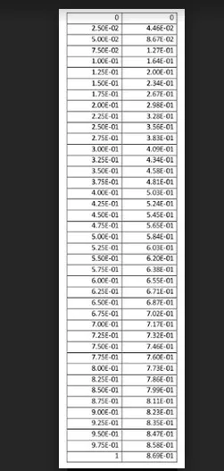
The above figure shows the data for hyperelastic material. Here we are going to import these data into the hyperelastic material and run the tensile test analysis to verify the stress-strain data and find the money constant using Mat 77 H and Ogden constant using material Mat 77 O.

Analysis:

Import the k file which contains the nodes and the elements. Since it is a shell element, specify this as 2d shell with a thickness 1.5 mm in the section.

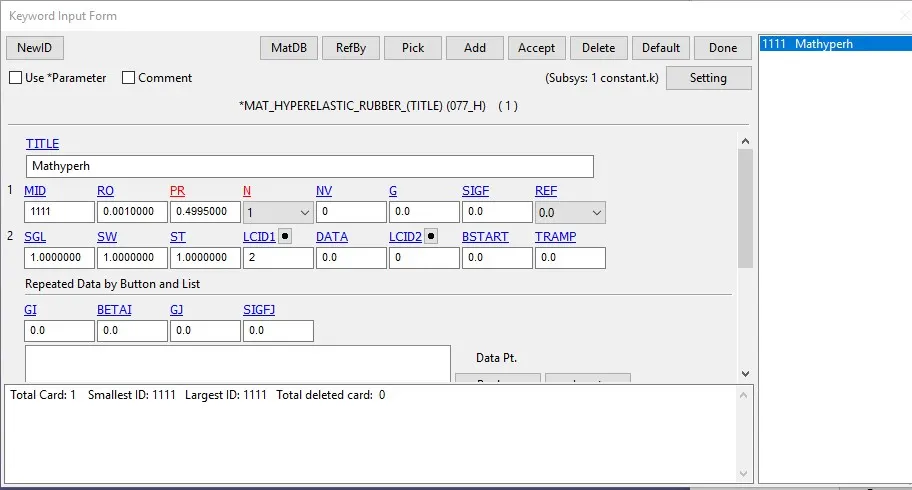
In material, Select the material as MAT 77 H- Hyperelastic material. Specify the value such as density, Poisson ratio,N , SGL, SW, and ST. Define the load curve.

Poisson Ratio:

We know the ratio of lateral strain to longitudinal strain is called as Poisson ratio. The Max value of the Poisson ratio is 0.5. If we use the value 0.5, then the volumetric strain we get is zero which means incompressible. But hyperelastic material is compressible with high strain rates. So in order to do the analysis, we need to specify the value of Poisson ratio less than 5. So we use the value of the Poisson ratio is 0.4995 to get the change in shape and do the analysis.

Similarly, the constant value is calculated based on the value of N. Implicitly this value N tells the degree of accuracy.

Load Curve:

Using the excel sheet to import the value of engineering stress and strain from the image. These values are defined as the load curve where the material behaves as a hyperelastic rubber.m To calculate Mooney constant use the MAT 77 H and to calculate the Ogden constant use MAT 77 0.

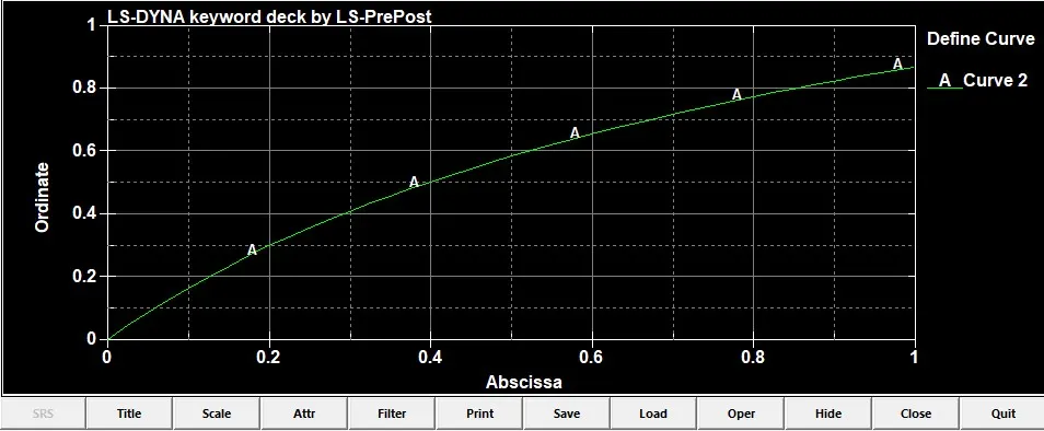
Once we create the section and the material specified in the part.

Boundary Condition:

Apply the essential and natural Boundary conditions to run the tensile test analysis.

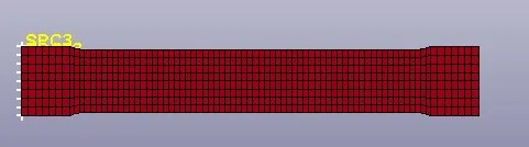
The above figure shows the boundary condition where the single point constraint is applied to all dof except translation in y.

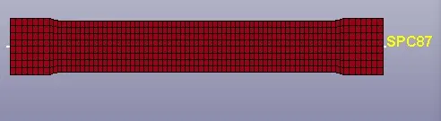
The above figure shows the boundary condition where SPC is applied on those two nodes which constrain only the translation y direction.

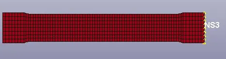
The above figure shows the Boundary condition where the displacement curve is applied by using the defined load curve.

Here we need to do the tensile test up to 100 percent strain.

100% strain = 1

Engineering strain = 1= change in length/original length

True Strain= ln(1+1)=0.6931.

Change in length= 0.6931 * original length

For the specimen, the initial length is 145.

so, the change in length is 100.

So, we need to define the load curve with the displacement of 100mm tensile to calculate the constant.

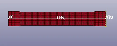
The above figure shows the initial length of the specimen.

Since the tensile test process is a slow process. For this, we will use implicit analysis.

Once we define all the boundary conditions. Import the file in LS Manage to run the analysis.

Result:

The above figure shows the final length of the specimen is 245mm. It means the strain value is 100%.

Stress and Strain Plot:

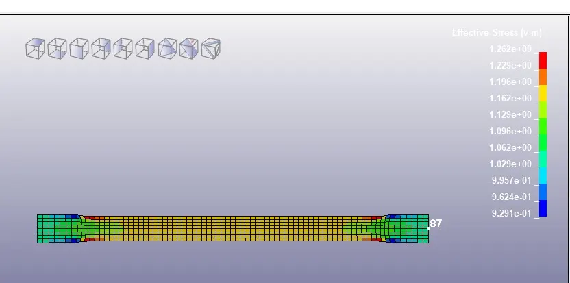
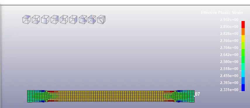
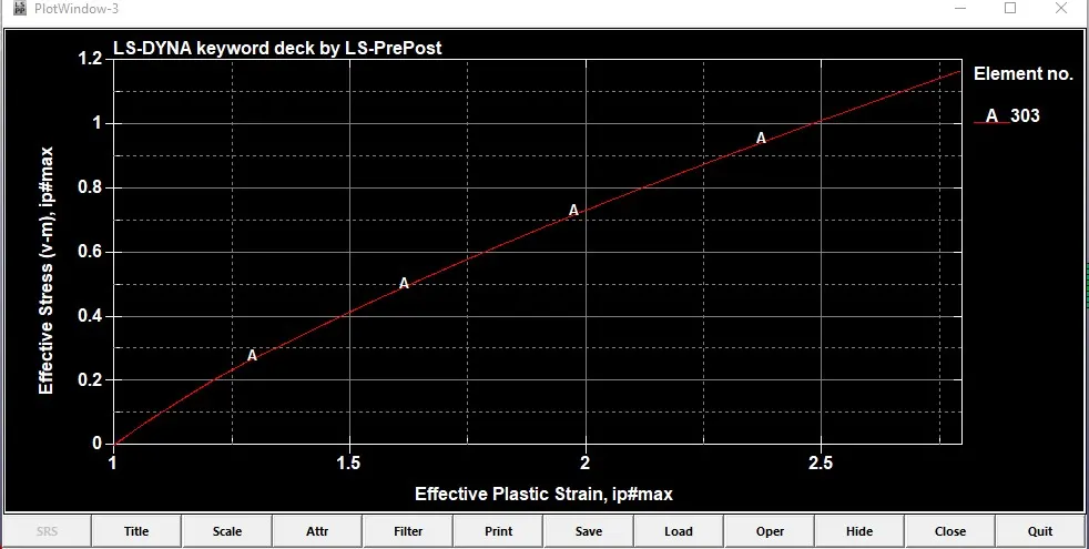
The above three figure shows the effective stress, effective plastic strain and stress-strain curve respectively. From the plot it clearly shows that this curve and the material given curve matches accurately.

Get the constant value and the stress value from the d3hsp file.

For N=1

Mooney constant C1=0.1768, C2=0.1474.

For N=2:

Mooney Constant:

Hyperelastic Constant C10= 0.2595E+00
Hyperelastic Constant C01= 0.4594E-01
Hyperelastic Constant C11= -0.2092E-01
Hyperelastic Constant C20= 0.2913E-02
Hyperelastic Constant C02= 0.1016E-02
Hyperelastic Constant C30= 0.0000E+00

For N=3

Hyperelastic Constant C10= 0.2611E+00
Hyperelastic Constant C01= 0.4420E-01
Hyperelastic Constant C11= -0.6076E-02
Hyperelastic Constant C20= -0.2667E-02
Hyperelastic Constant C02= -0.9966E-02
Hyperelastic Constant C30= 0.1565E-03

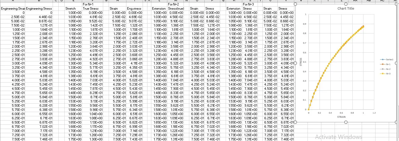
From the above excel sheet and the graph, the analysis and the values of the given materials are verified.

Ogden Constant:

To get the constant value of Odgen we will use the same analysis except the material MAT 77H. Here we use the Material MAT 77 O.

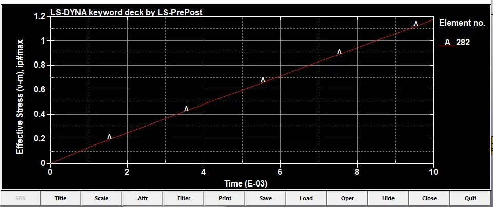
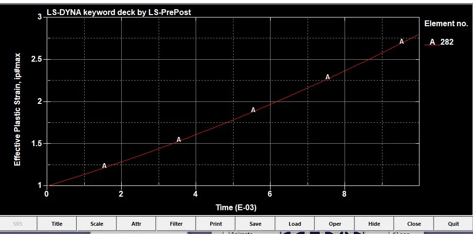
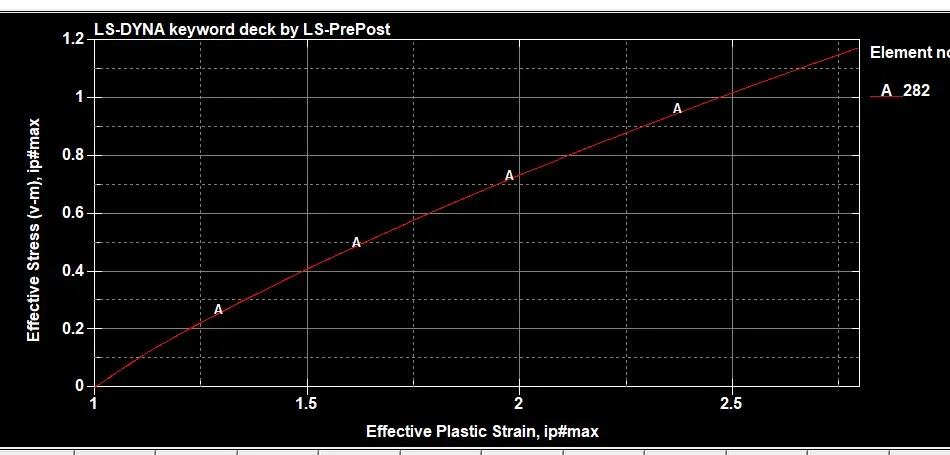
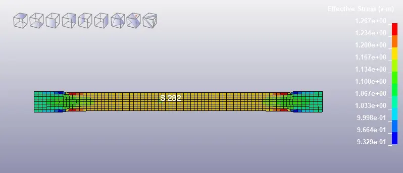
From the above result, the result we get in the MAT 77H and here MAT 77 O is more or less same.

Constant Value:

Here we have N value up to 8. But for comparing purposes we limit up to 3.

For N=1

mu(1)= 9.1076025585232E-01 alpha(1)= 1.3427238694706E+00

For N=2

mu(1)= 9.1564733498464E-01 alpha(1)= 1.3399091807896E+00
mu(2)= 2.2259556593837E+00 alpha(2)=-1.8434703015661E-03

For N=3

mu(1)=-3.1842608038997E-02 alpha(1)= 1.9263175501595E+00
mu(2)= 2.6137537530451E-01 alpha(2)= 1.5503338135517E+00
mu(3)= 6.8199188165234E-01 alpha(3)= 1.2887845124363E+00

Conclusion:

Thus the given material data is imported in the hyperelastic model to run the tensile test analysis and the value of the given stress and strain are verified.