Week - 10 Hyperelastic Material Models

Hyperelastic Material Models

Aim: To create a Hyperelastic material model using MAT 077 H_Hyperelastic rubber using Mooney Rivlin & Ogden law and compare its value with respect to the provided Engineering Stress & Engineering Strain in the form of graph.

All units used here are in Kg mm ms.

Steps followed:

Case 1: Mooney Rivlin law used with Number of constants(N) to solve the function of Engineering Stress vs Engineering Strain Graph=1

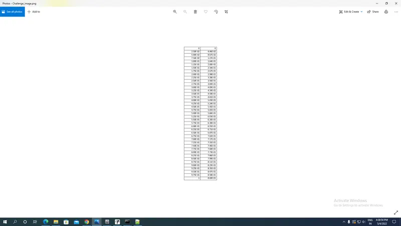
• Download the data of Engineering stress(MPa) and Engineering Strain(mm/mm) as shown in the image below:

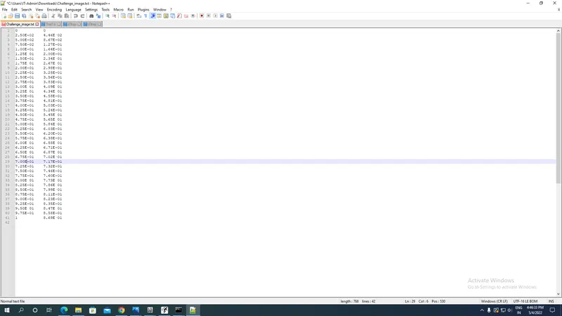
• Convert the image .png file to TXT format and open it in notepad++ format as shown in the image below with all datas:

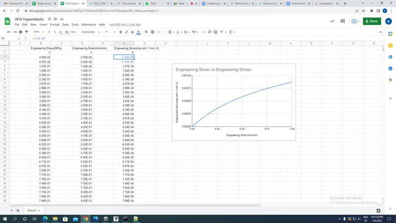
• Copy all the Datas to the excel sheet with True stress and convert it into Kg mm^-1 ms^-2 by multiplying stress with 1E-03 as shown in the image below:

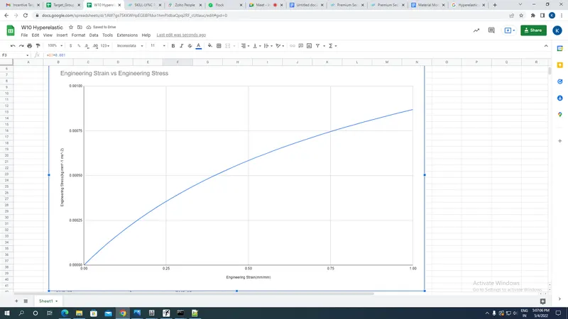
• Plot the Engineering Stress vs Engineering Strain as shown in the image below:

• Now we will open the LS Prepost and import the Dogbone file provided in the question in .k format as shown below by selecting import options under Files and selecting Keyword files after downloading the file.

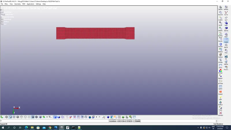
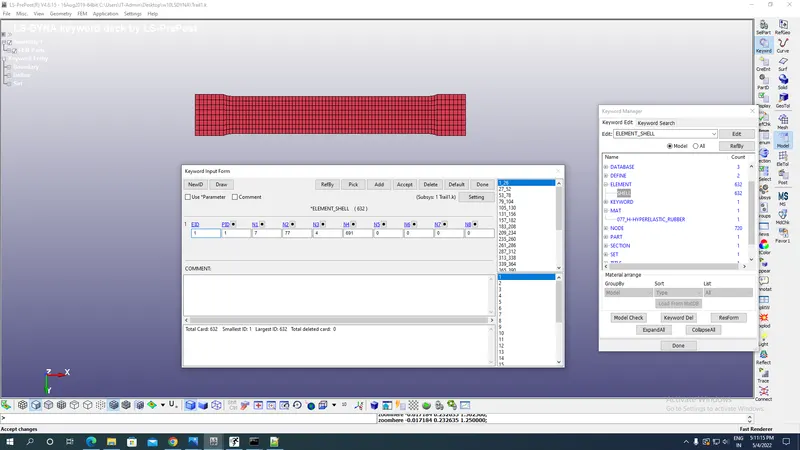
• Now as this model is already provided with Geometry & shell type elements we have to define the section,materials,parts,boundary condition,types of solvers(Explicit or Implicit),Termination Time,Database outputs & curves.

• Now we check the type of element under the Keyword option in Models in the left side Toolbar as shown in the image below with particular shell Id,part Id etc.

• Section:

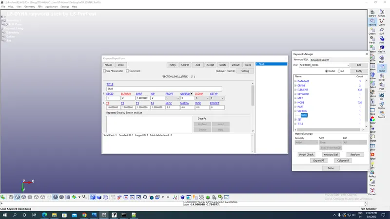
Now create section for Dogbone specimen with appropriate section id, which is in almost 2D geometry as we know for that we have to create a shell section of it with appropriate Element formulation of 2 which is Belytschko-Tsay membrane which is fully integrated & Ideal for fabrics with negligible bending stiffness and at the same time this formulation is economical. Shell thickness is taken as 1 mm as shown in the image below:

• Material selection:

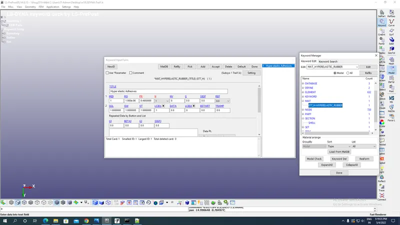
Now select the MAT- 077 H_Hyperelastic_Rubber material for Dogbone specimen under Mat keyword by going into Toolbar at right containing Model and from there Keyword & from there to MAT- 077 H_Hyperelastic_Rubber material.ThisMAT- 077 H_Hyperelastic_Rubber material material is chosen with density of Graphite as 0.000001 kg/mm^3, Poisson's ratio as 0.495 so that we can observe deformation of Dogbone specimen upon UNIAXIAL tension test. Now we are taking Number of Constants to solve Engineering Stress vs Strain graph(N) as 1 which gives us 2 constants as C01 & C10 with Specimen Gauge Length,Thickness & width all as 1 because we are inserting directly Engineering Stress vs Strain curve in LCID 1 so we don’t require dimensions until & unless we have that Force vs Displacement curves.

• Now we have to define the Load ID curve for LCSS which we are going to do by Define curve option & inserting 0,0 for Engineering stress & Engineering Strain.

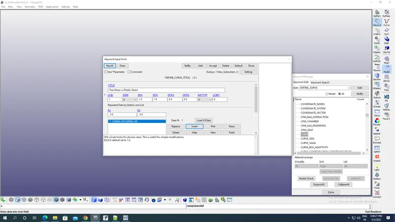
• Now save the model you have edited & close it,go to excel sheet & select all the Positive Effective Plastic strain and their respective true stress in GPa and copy them.Negative Plastic strain is not taken because it indicates only True Elastic strain from which we can get Young’s modulus but as here Young’s Modulus is given we are interested in calculating the effect of true stress after Elastic part i.e Plastic part.
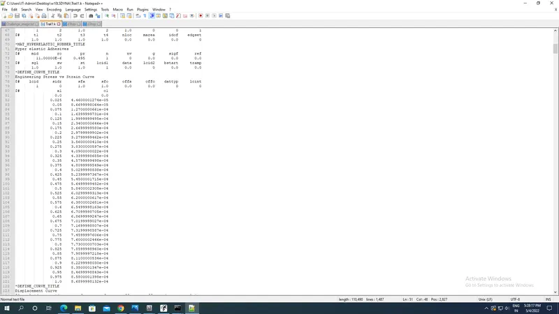
• Open the save .k file of model in Notepad++ and try pasting the Engineering strain & Engineering stress in LCSS by removing the 0,0 which have been provided earlier as shown in the image below:

• Parts creation:

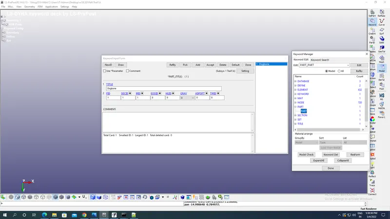
Now the parts which are there after Geometry are assigned with section &, material Id under Part option keyword by going into Toolbar at right containing Model and from there Keyword & from there to Part by assigning section id,material id,part id & Part title as shown in the image below:

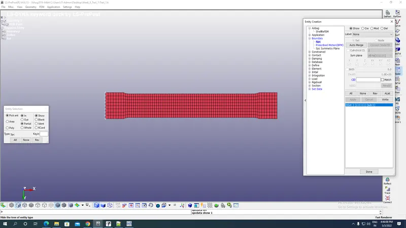
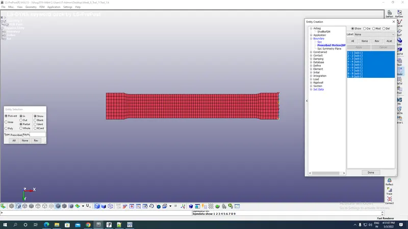
• Now define Boundary SPC for fixing the one side with the help of Create Entity Boundary SPC as shown below by selecting nodes properly as shown in the image below:

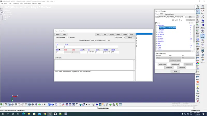
• Now define the Prescribed Rigid Motion in Boundary conditions with the help of Create Entity Boundary Conditions with help of Displacement by knowing the Strain at the last point i.e. 4.43E-03 X 145mm length of Dogbone Specimen which is 0.64 mm displacement with DOF=1 Translational along X axis.

We are applying this for displacement along X-axis.

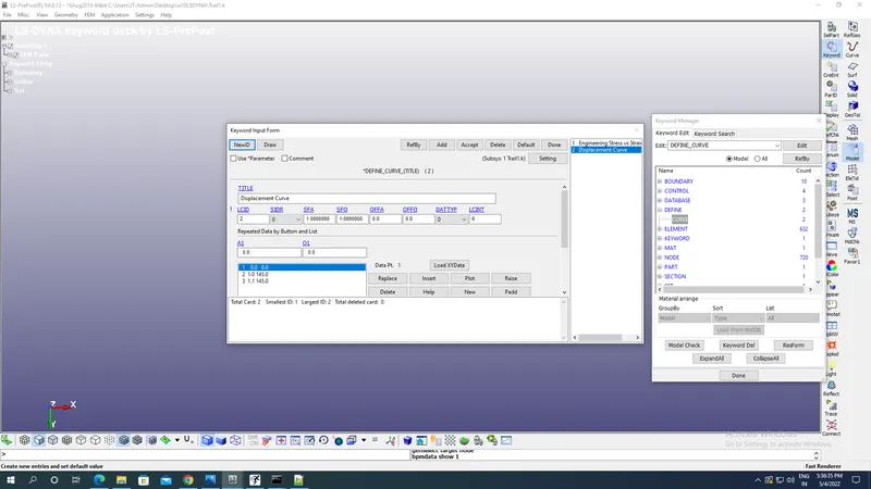
• Now Define displacement curve by inserting Displacement vs Time graph for 0 ms to 0 mm then at 1 ms its 145 mm and 1.1 ms to 145 mm again because its mentioned in the data of Engineering Strain provided above that it should be 100% or 1(mm/mm) and length of dogbone specimen is 145 mm so maximum displacement should be 145X1=145mm.

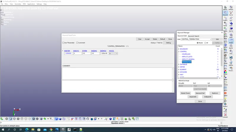
• Now go to Control-Termination and apply End time of 1 ms as shown in the image below for our simulation.

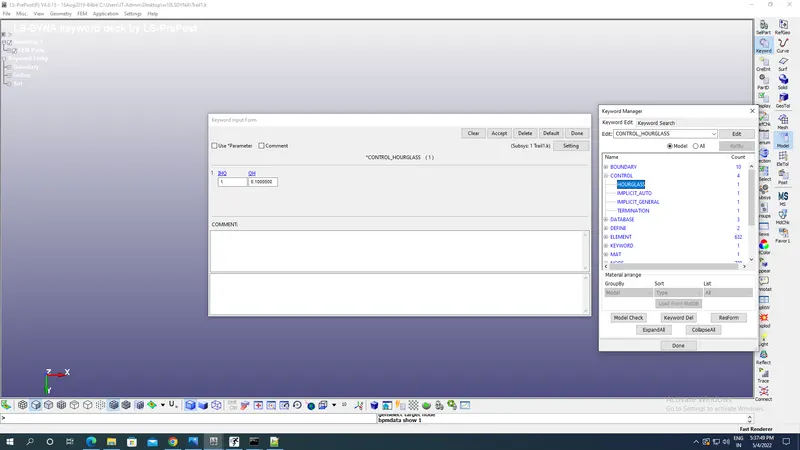
• Now apply Hourglass for shell elements so that we can calculate the deformations not captured in the form of hourglass energy.For IHQ=1 we have Hourglass control is viscosity or stiffness that is added to quadrilateral shell elements and hexahedral solid elements that use reduced integration. It also applies to formulation 1 tshells. Without hourglass control, these elements would have zero energy deformation modes which could grow large and destroy the solution. CONTROL_HOURGLASS can be used to redefine the default values of the hourglass control type and coefficient. If omitted or if IHQ = 0, the default hourglass control.

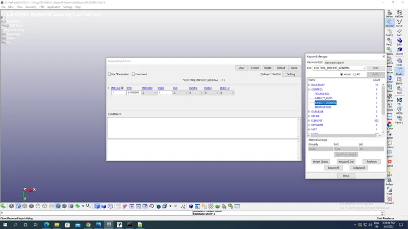
• Now we are taking Implicit solver for our simulation with Implicit general card as this tensile test of Dogbone is almost time independent or Quasi Static process.
• We are using Implicit general card with IMFLAG=1 for Implicit Analysis with Initial Time step size as 0.1 ms as shown in the image below:

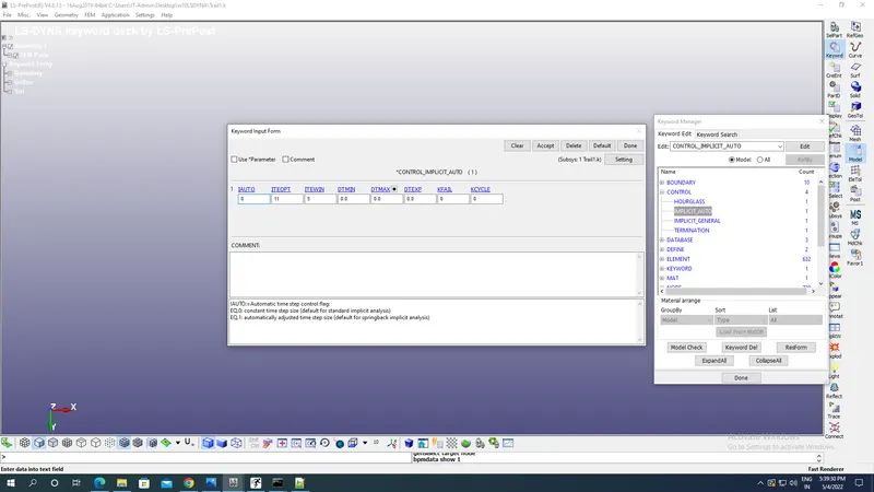
• Now Implicit auto is used for Define parameters for automatic time step control during implicit analysis with IAUTO=0 for constant Time step size ,ITEWIN=11 & ITEOPT=5 as shown in the image below:

Output Requests:

• Now we are going to request for our outputs with DATABASE-ASCII-GLSAT for showing various energies while MATSUM for material internal energies as shown in the image below with Time interval between outputs(DT) as 0.1 ms:

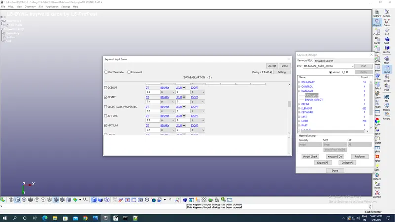
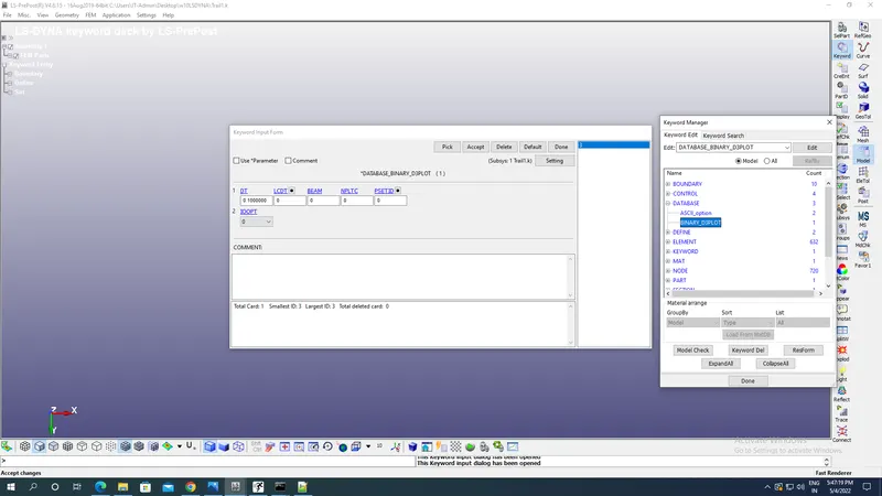
• For Binary d3plot we even keep DT same as 0.1 ms as shown in the image below:

Results:

X stress d3plot:

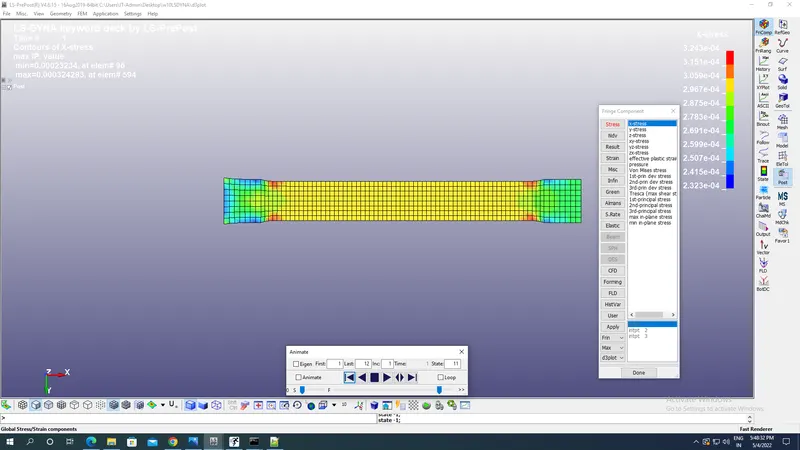
Maximum X stress= 3.243E-04GPa.

Elastic strain along X axis:

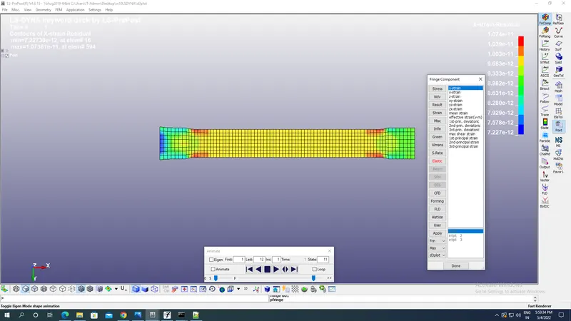
Maximum Elastic strain=1.047E-11 at element number 594.

Now we will open d3hsp in notepad++ and we will look for Mooney Rivlin two constants which are shown below having values of C01=0.1768E-03 & C10 =0.1474E-03

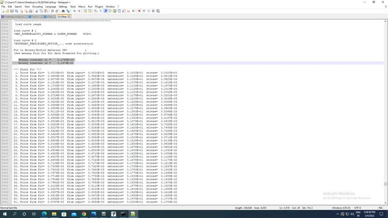
Now we will look below Mooney constants for our True Stress & Stretch values and copy them in our excel sheets as shown below:

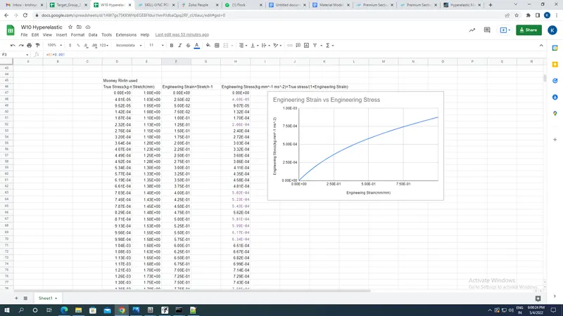
Now will obtain from stretch our Engineering Strain in(mm/mm) as Engineering Strain=Stretch-1 and Engineering stress=True stress/(1+Engineering Strain) by our formulas:

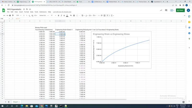
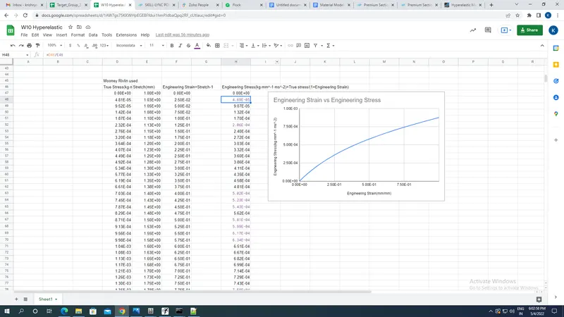
Plot the Engineering Stress vs Engineering Strain graph appears as shown:

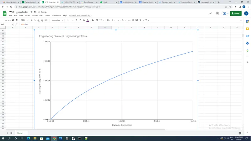
Case 2: Ogden law used with Number of constants(N) to solve the function of Engineering Stress vs Engineering Strain Graph=3.

Steps followed:

All the steps to be followed are similar to case 1 only number of solver required to solve Engineering stress vs Strain(N)=3 in Material card as in Ogden law we have 6 constants as shown in the image below:

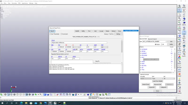
All boundary conditions,meshing,parts,section & Termination time output request remains same as in case 1.

Results:

X stress d3plot:

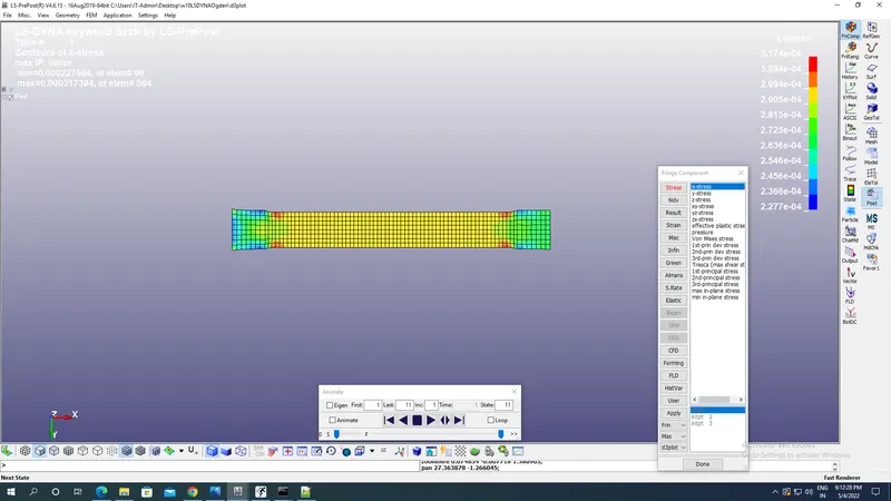
Maximum X stress= 3.174E-04GPa.

Elastic strain along X axis:

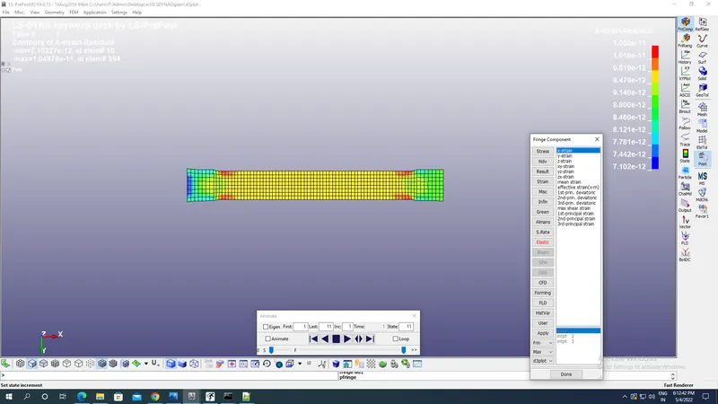
Maximum Elastic strain=1.050E-11 at element number 594.

Now we will open d3hsp in notepad++ and we will look for Ogden six constants which are shown below having values:

Hyperelastic Constant C10= 0.2611E-03

Hyperelastic Constant C01= 0.4420E-04

Hyperelastic Constant C11= -0.6077E-05

Hyperelastic Constant C20= -0.2666E-05

Hyperelastic Constant C02= -0.9966E-05

Hyperelastic Constant C30= 0.1565E-06

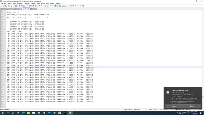
Now we will look below Ogden constants for our True Stress & Stretch values and copy them in our excel sheets as shown below:

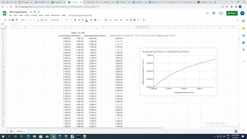
Now will obtain from stretch our Engineering Strain in(mm/mm) as Engineering Strain=Stretch-1 and Engineering stress=True stress/(1+Engineering Strain) by our formulas:

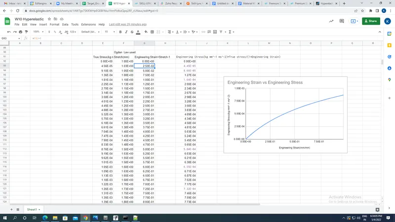
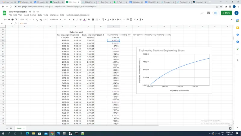
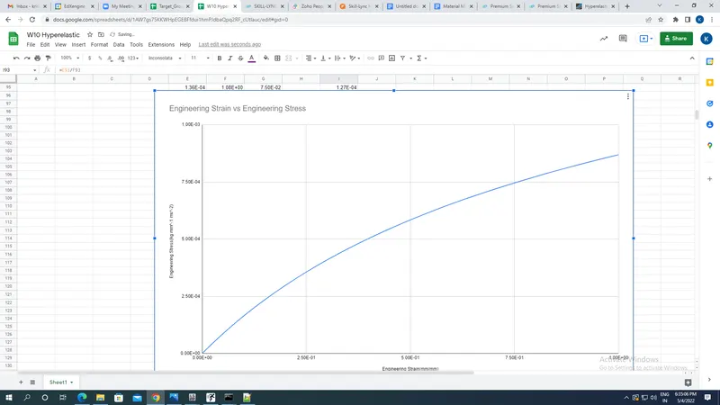
Plot the Engineering Stress vs Engineering Strain graph appears as shown:

Comparison of Case 1& 2 with Engineering stress & strain:

At strain 2.50E-01:

Provided Engineering Stress:3.56E-04

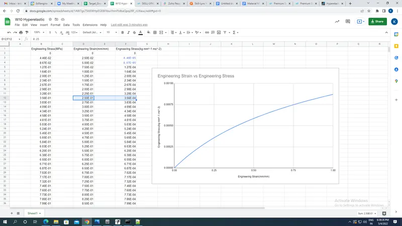
CASE 1:Mooney Rivlin law applied on Hyperelastic material:

At strain 2.50E-01:

Provided Engineering Stress:3.60E-04

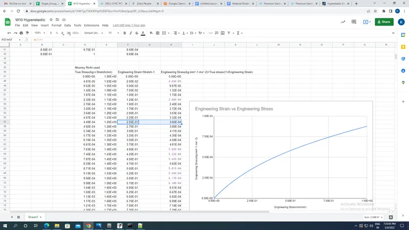
CASE 2:OGDEN law applied on Hyperelastic material.

At strain 2.50E-01:

Provided Engineering Stress:3.56E-04

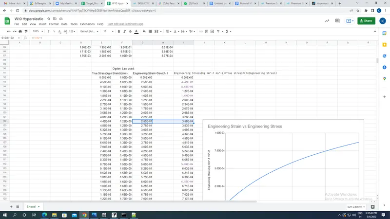
So from the plot at 2.50E-01 Engineering strain of Engineering stress in Hyperelastic material with Ogden law we can observe that its value is close to the reference value of Engineering Stress provided so Ogden law is more accurate compared to Mooney Rivlin law for hyperelastic materials.

Conclusion:

Material Modeling is done for Mat 077 H_Hyperelastic material using Mooney Rivlin & Ogden law and values of Engineering stress is compared at a particular strain and we found that Hyperelastiuc material with Ogden Law is more accurate than Mooney Rivlin.