Week 1- Mixing Tee
Objective:
The objective of the project is to perform steady state simulation to determine the mixing effectiveness when hot air with temperature 36°C mixes with the cold air with temperature 19°C in mixing tee joint.
The results must be provided for following conditions:

The required images from the simulation:

And convergence plot of each simulation.
Design Inputs:
- Mixing Tee CAD models for both short & long length
- Hot air inlet speed & temperature and cold air temperature
Model for simulation:
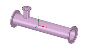
Given model:
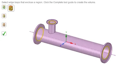
Using Volume Extract command, the inner volume of the fluid has been extracted. Following image shows the selected edges to extract the inner fluid volume from the Mixing Tee model.
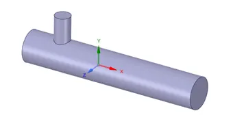
The resulted model which will be used for the simulations is showcased as follows:
Meshing:
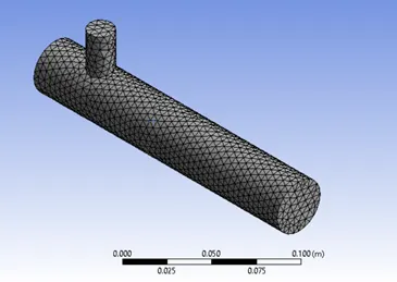
The meshing has been performed with the default options except the size of the elements which will be kept at the 0.0045m. The mesh has 13962 elements.
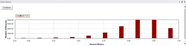
The quality of the mesh is displayed in the following figure.
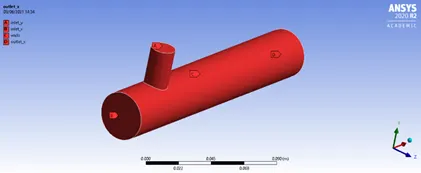
The selected faces have been given name for identification purpose while setting up the simulation.
Simulation Setup:
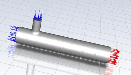
The model has been imported into the fluent. The image shows the model with the initial boundary conditions with the hot & inlet fluid temperature and the fluid velocity. The blue arrows display the inlet while the red ones display the outlet.
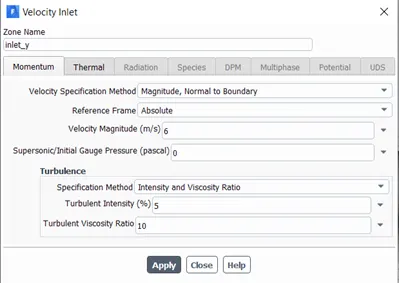
The boundary conditions for the simulation have been inserted using the boundaries tab available into the Physics menu. In following image, the velocity has been inserted into the velocity magnitude & fluid temperature into the next tab called Thermal. In the similar way the information for hot & cold fluid has been inserted for all simulations.
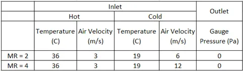
Following table shows the information regarding the temperature, velocity & gauge pressure used for each simulation for inlet & outlet as part of boundary conditions.
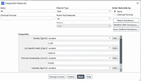
Default air material with the default properties has been used.
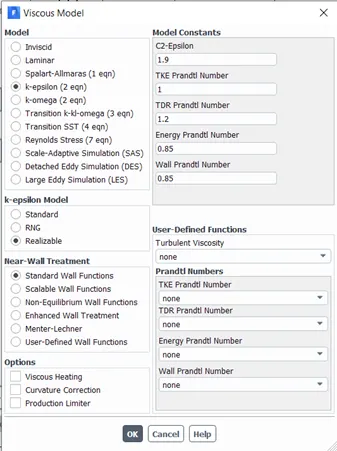
Viscous model has been selected from the viscous model selection dialogue box accessed from the Physics tab. The selected k-epsilon model has been displayed in the following image & the k-omega SST has been used.
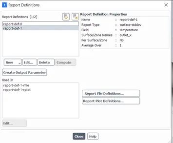
Additional two reports to extract information about the temperature distribution on the outlet face of the mixing tee, the Area weighted average of temperature & standard deviation reports has been setup from the definition tab available in Solution > Report tab.
The simulation process has been initialized after selecting Hybrid method. The hybrid method will help in approximating the pressure & velocity information of the fluid.
The number of iterations has been set as 300.
The above-mentioned process has been followed for all simulations.
Results / Post Processing:
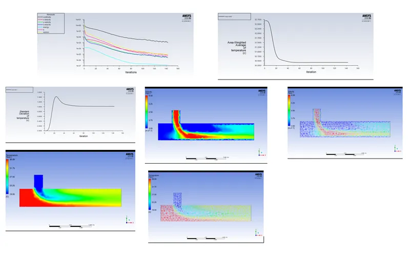
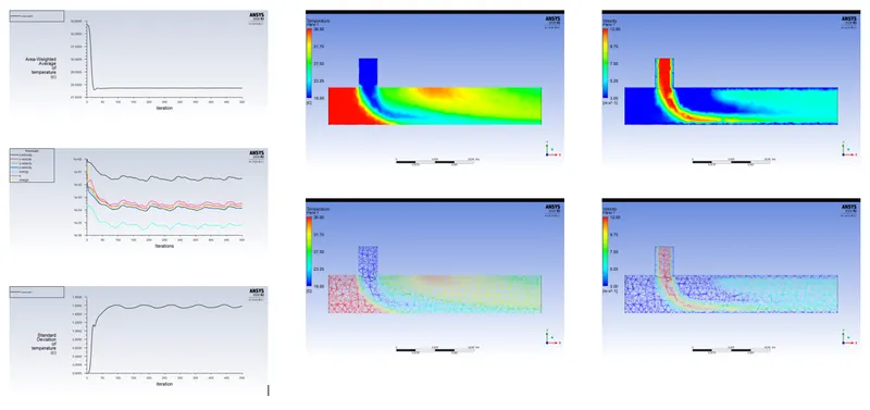
1. Case 1:
MR = 2, Viscous Model = K-epsilon Realizable with Standard Wall Treatment
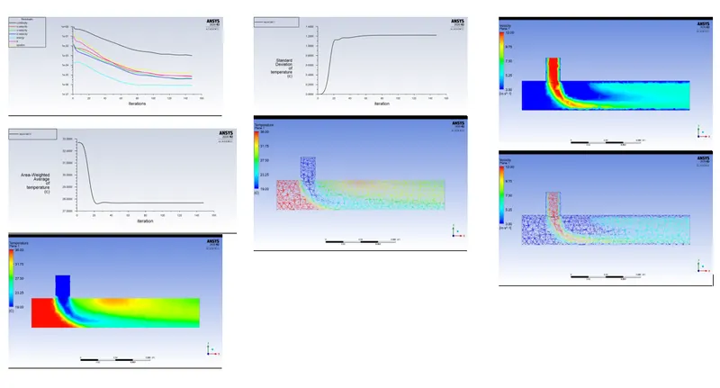
2. Case 1:
MR = 4, Viscous Model = K-epsilon Realizable with Standard Wall Treatment
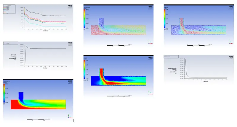
3. Case 1:
MR = 2, Viscous Model = K-omega SST
4. Case 1:
MR = 4, Viscous Model = K-omega SST
K-epsilon vs k-omega SST Viscous Model:
k-epsilon:
The baseline two-transport-equation model solving for kinetic energy k and turbulent dissipation ε. Turbulent dissipation is the rate at which velocity fluctuations dissipate. This is the default k–ε model. Coefficients are empirically derived; valid for fully turbulent flows only. The k-e model uses the gradient diffusion hypothesis to relate the Reynolds stresses to the mean velocity gradients and the turbulent viscosity. Performs poorly for complex flows involving severe pressure gradient, separation, strong streamline curvature. The most disturbing weakness is lack of sensitivity to adverse pressure gradients; another shortcoming is numerical stiffness when equations are integrated through the viscous sublayer which are treated with damping functions that have stability issues.
k-omega SST:
A two-transport-equation model solving for kinetic energy k and turbulent frequency ω. This is the default k–ω model. This model allows for a more accurate near wall treatment with an automatic switch from a wall function to a low-Reynolds number formulation based on grid spacing. Demonstrates superior performance for wall-bounded and low Reynolds number flows. Shows potential for predicting transition.
Shear Stress Transport (SST) is a variant of the standard k–ω model. Combines the original Wilcox k-w model for use near walls and the standard k–ε model away from walls using a blending function, and the eddy viscosity formulation is modified to account for the transport effects of the principle turbulent shear stress.
The SST variant of the k-omega has advantage of both standard k-omega & k-epsilon model. That’s why for the Case 2, k-omega SST model will be used.
5. Case 2:
MR = 2, Viscous Model = K-omega SST
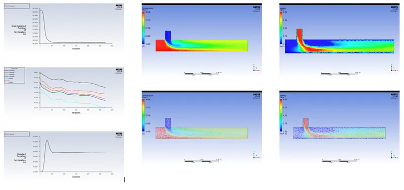
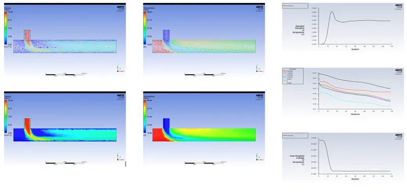
6. Case 2:
MR = 4, Viscous Model = K-omega SST
Results Table:
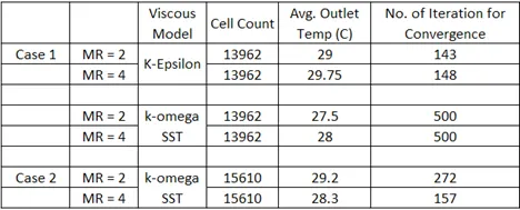
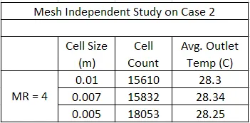
Mesh Independent Study: