Week 1- Mixing Tee
AIM:
to create the steady state simulation to compare the mixing effectiveness when hot inlet temperature is 36-degree Celsius and cold inlet temperature is 19-degree Celsius for two cases (long mixing tee and short mixing tee)
INTRODUCTION
- turbulent mixing of fluid of different temperature in T junction geometries became of significant important in many fields.
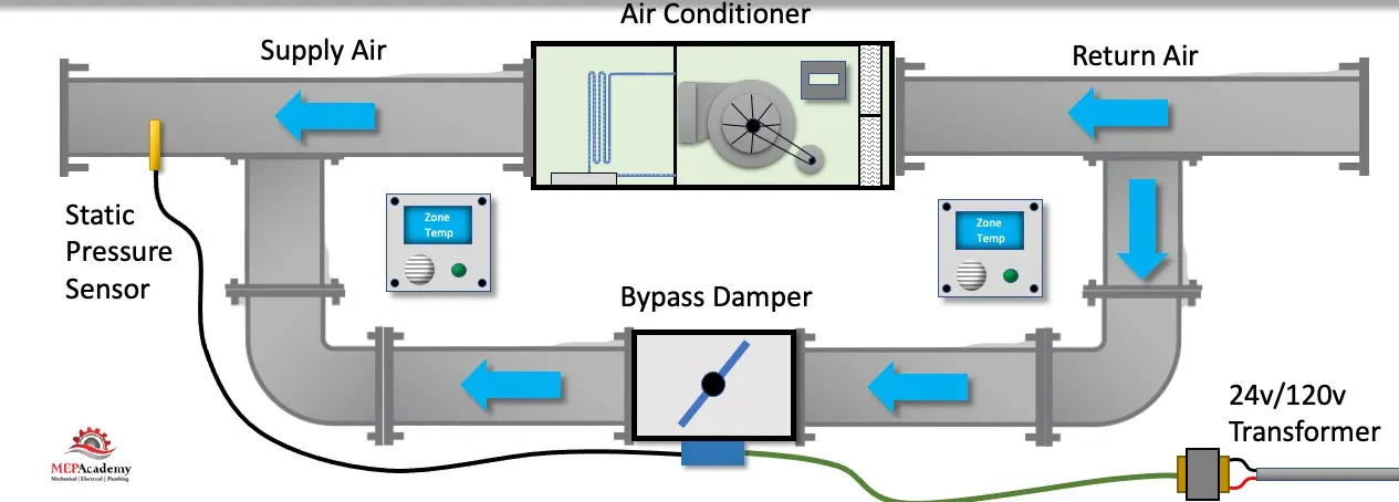
- In the case of HVAC systems, bypass mechanism at T junction play a crucial role in enhancing energy efficiency and optimizing airflow distribution.
- By allowing a controlled portion of air or fluid to bypass certain components, these systems help maintain balanced temperature distribution while reducing unnecessary energy consumption.
- In air handling units, a bypass at a T junction can mix return and supply air to minimize excessive heating or cooling loads, improving overall efficiency.
- effective design of T junction bypass reduces fan and pump workload, prevents thermal stratification and enhances system longevity.
- utilizing CFD analysis engineers can optimize bypass configuration to achieve uniform mixing, reduces energy waste and maintain indoor comfort while maximizing HVAC system efficiency.
ANALYTICAL SOLUTION: (MASS WEIGHTED AVERAGE APPROACH)
Tmixture is used to find the temperature for the complete mixing that the two fluid streams are fully blended immediately after the T-junction.

H enthalpy is the measure of total energy in the system including both its internal energy and the energy required to displace its surrounding
H = U + PV
where,
U is the internal energy
P is the pressure
V is the specific volume
for ideal gases, enthalpy will be
H = cp dtT
where,
cp is the specific heat at constant pressure
dtT is the temperature difference i.e. actual temperature - reference temperature (25-degree Celsius)
Hmixture is used to find the enthalpy for the complete mixing that the two fluid streams are fully blended immediately after the T-junction

- Hot air temperature = 36 degree Celsius = 309 K
- Cold air temperature = 19 degree Celsius = 292 K
mass of hot air, m = Q * ρ
wkt, Q = V * A
Where,
Q is the volume of air
ρ is the density of air
V is the Velocity of air
A is the area of the pipe in which air is flowing
CASE 1 ( mometum ratio = 2)
momentum ratio = velocity of cold inlet / velocity of hot inlet
Given data:
velocity of hot inlet = 3 m/s
dia of the pipe = 0.0338761 m
from momentum ratio, the velocity of cold inlet = 6 m/s
- mass of hot air, mhot = (3.14/4) * 0.03387612 * 3 * 1.225 = 0.0033106 Kg/m-s
- mass of cold air, mcold = (3.14/4) * 0.01696262 * 6 * 1.225 = 0.0016601 Kg/m-s
for the above formula, for Tmixture
Tmixture = [(0.0033106 * 309) + (0.0016601 * 292)] / (0.0033106 + 0.0016601)
Tmixture = 301.3243 K
- enthalpy of hot air, Hhot = 1005 * (309 - 298) = 11055 J/kg
- enthalpy of cold air, Hcold = 1005 * (292 - 298) = -6030 J/k
for the above formula,
for the above formula, for Hmixture
Hmixture = [(0.0033106 * 11055 ) + (0.0016601 * -6030)] / (0.0033106 + 0.0016601)
Hmixture = 5349.0011 J/kg
to find the length of the pipe to get completely mixed:
Vmixture = [(0.0033106 * 3) + (0.0016601 * 6)] / (0.0033106 + 0.0016601)
Vmixture = 4.0019 m/s
Re = (ρ*V*D)/μ
μ - dynamic viscosity
Re = (1.225 * 4.0019 * 0.0338761)/ 1.851 x 10^-5
Re = 8972 - turbulent
le = 4.4 * Re(1/6) * D
le = 4.4 * 8972(1/6) * 0.0338761
le = 0.679 m
This means the two air streams will fully mix after traveling approximately 0.679 meters downstream of the T-junction.
CASE 2 ( mometum ratio = 4)
momentum ratio = velocity of cold inlet / velocity of hot inlet
Given data:
velocity of hot inlet = 3 m/s
dia of the pipe = 0.0338761 m
from momentum ratio, the velocity of cold inlet = 12 m/s
- mass of hot air, mhot = (3.14/4) * 0.03387612 * 3 * 1.225 = 0.0033106 Kg/m-s
- mass of cold air, mcold = (3.14/4) * 0.01696262 * 12 * 1.225 = 0.00332025 Kg/m-s
for the above formula, for Tmixture
Tmixture = [(0.0033106 * 309) + (0.00332025 * 292)] / (0.0033106 + 0.00332025)
Tmixture = 300.4876 K
- enthalpy of hot air, Hhot = 1005 * (309 - 298) = 11055 J/kg
- enthalpy of cold air, Hcold = 1005 * (292 - 298) = -6030 J/kg
for the above formula,
for the above formula, for Hmixture
Hmixture = [(0.0033106 * 11055) + (0.00332025 * -6030)] / (0.0033106 + 0.00332025)
Hmixture = 2500.0679 J/kg
to find the length of the pipe to get completely mixed:
Vmixture = [(0.0033106 * 3) + (0.0016601 * 12)] / (0.0033106 + 0.0016601)
Vmixture = 6.0057 m/s
Re = (ρ*V*D)/μ
μ - dynamic viscosity
Re = (1.225 * 6.0057 * 0.0338761)/ 1.851 x 10^-5
Re = 13464 - turbulent
le = 4.4 * Re(1/6) * D
le = 4.4 * 13464(1/6) * 0.0338761
le = 0.727 m
This means the two air streams will fully mix after traveling approximately 0.727 meters downstream of the T-junction.
ANSYS FLUENT SETUP: (NUMERICAL APPROACH)
SPACECLAIM:
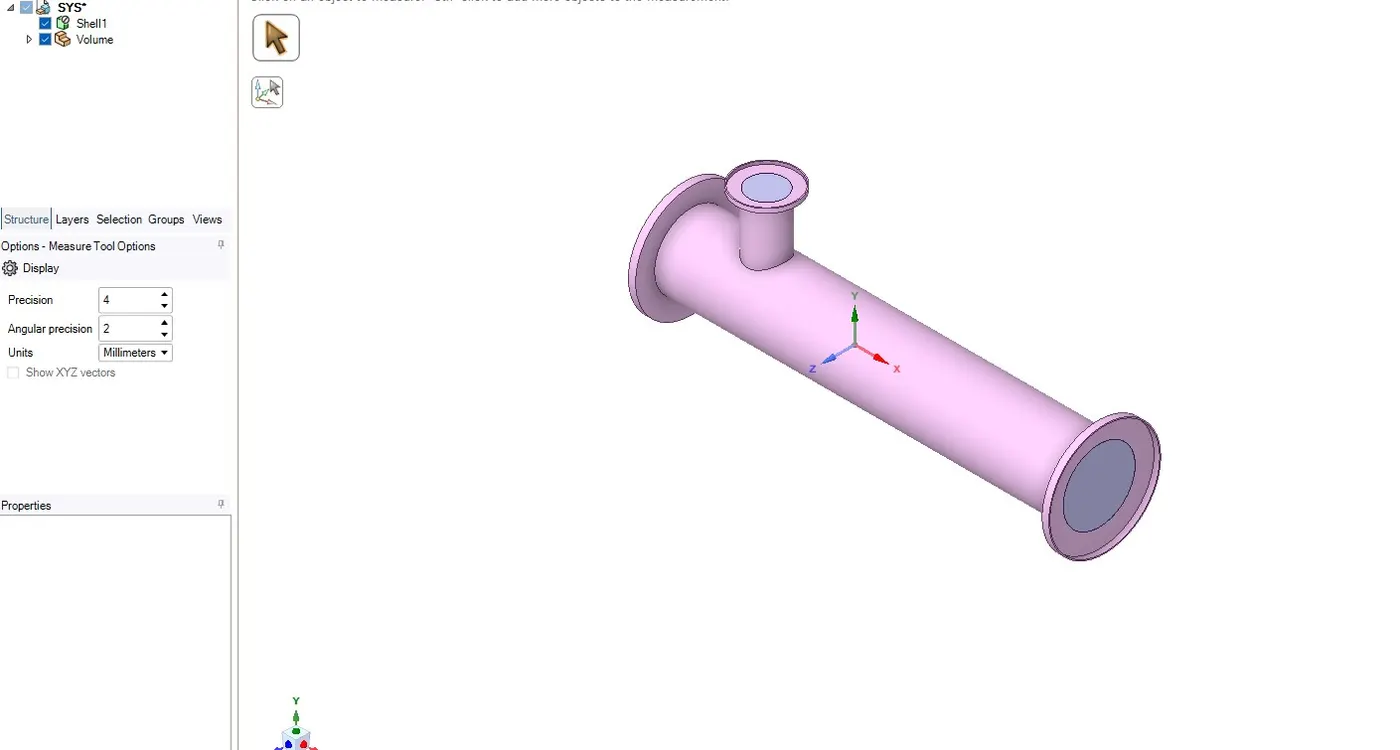
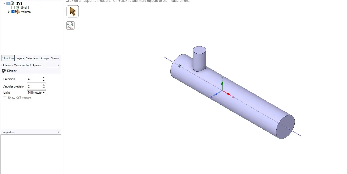
- from the given model, the unnecessary features like pipe flanges need to be eliminated and as it is a flow problem not a heat transfer through pipe, it is better to make as a full solid in the pipe element using volume extract option. where we will be meshing in the solid volume to capture the fluid flow using discretization
- Updated model after suppressing the shell body.
MESHING:
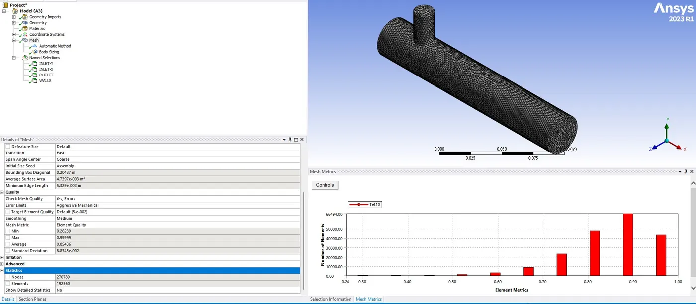
- the mesh used here is tetrahedral
- element - 192360
- node - 270789
- name selection is created for all the boundary and initial conditions
FLUENT (ANALYSIS SETUP)
Types of solvers:
- Pressure based solver
- Density based solver
Incompressible flow - density remains constant. solving for pressure and velocity relationship
Compressible flow - density changes significantly due to pressure and temperature
Pressure based solver:
- the continuity equation for incompressible fluid does not include density changes. instead, it simplifies to
∇⋅V=0
- This means mass conservation (continuity equation) only ensures velocity correction but does not directly relate to pressure.
- since pressure is still needed to drive the flow, we must use pressure correction algorithms to adjust velocity and pressure fields iteratively.
Density based solver:
- the continuity equation includes density as a variables
(∂ρ/∂t) +∇⋅(ρV)=0
- now density changes with pressure and temperature, so we can no longer assume it as constant. instead of solving for pressure separately, we solve for density directly along with momentum and energy equations
- this naturally links pressure, velocity and temperature, making a density-based solver more efficient for compressible flows
as we discussed about the usage of the solvers. in this analysis we are using incompressible flow thus we are going with pressure-based solver.
Velocity formulation:
when dealing with fluid flow in rotating and stationary reference frames, we can use two types of velocity formulation
- Absolute velocity formulation
- relative velocity formulation
Absolute velocity formulation:
- absolute velocity is measure relative to a fixed (inertial) reference frame
- it represents the actual velocity of the fluid in space
- used in stationary component system like airflow in an HVAC duct
Relative velocity formulation:
- relative velocity is measure relative to a rotating reference frame
- It accounts for motion with respect to the moving part of system
- used in rotating machinery (e.g.: fans, turbines, HVAC blowers)
As disused above. this problem implies the stationary component like HVAC duct. Thus, we will use the absolute velocity formulation
Time based solver:
- steady state solver
- transient solver
T- junction mixing can be steady state if inlet velocities and temperature are constant over time, leading to a stable mixed flow
It becomes transient if inlet condition changes or unsteady effect like vortex shedding occur.
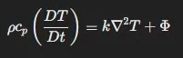
Energy equation:
- We use the energy equation because temperature is derived from energy conservation.
- It helps track heat transfer and temperature distribution in a system.
where,
ρ- density
Cp - specific heat capacity
T - temperature
k - thermal conductivity
Φ - viscous dissipation term (conversion of mechanical energy to heat)
Viscous model:
1) Inviscid model
- assumes the fluid has zero viscosity (ideal fluid)
- only solves the Euler equation (ignores shear stresses)
- used when external aerodynamics at very high Re number
- supersonic flows where viscosity effects are secondary
2) Laminar model
- solves the full Navier stokes equation without turbulence modelling
- assumes the flow is smooth and orderly (low Reynolds's number)
- used when flows at low Reynolds number, microfluidics and study slow-moving fluids
3) Spalart - Allmaras model (1 equation model)
- solves a single transport equation for turbulent viscosity
- developed for aerospace and external aerodynamic (airfoils, wings)
- less computationally expensive than two equation models
- used when external aerodynamics and for streamlined bodies
4) K-epsilon model (2 equation model)
- uses two equations for turbulence properties
- k (turbulent kinetic energy)
- epsilon (dissipation rate of turbulence)
- works well for high Reynolds number flows
variations of k-e model
Standard K-epsilon model:
- basic version assumes fully turbulent flows
- not very accurate for near wall flows
RNG k-epsilon model
- uses renormalization group (RNG) theory for improved accuracy
- better for low Reynolds number flows, swirling flows and separated flows
Realizable K-epsilon model
- modifies the turbulent viscosity formulation
- works well for flow with curvature, separation and strong swirling
used for good balance between accuracy and computational cost
industrial flows, HVAC, combustion, jet flows
5) k-omega model (2 equation model)
- similar to k-epsilon but uses omega (specific dissipation rate) instead of epsilon.
- better near walls than k-epsilon
variation of k-omega model
standard k-omega model:
- good for near wall prediction but too sensitive to freestream conditions
shear stress transport (SST) K-omega model
- hybrid model uses k-omega near walls and k-epsilon in the freestream
- more accurate for separated flows, adverse pressure gradients.
used when external aerodynamics, turbomachinery, and automotive industries.
6) Transition k-kl-omega model (3 equation model)
- adds an extra equation for laminar to turbulent transition prediction
- more accurate for cases where natural transition occurs
- used in turbine blades, airfoils application where transition prediction is critical.
7) transition SST model (4 equation model)
- more advanced version of SST k-omega
- includes additional transport equation for transition onset
- more reliable for boundary layer transition predictions
- used for high accuracy simulation of airfoils, blades, wings
8) Reynolds stress model (RSM) (7 equation model)
- solves separate transport equations for each Reynolds stress component
- more detailed than k-epsilon and k-omega
- best for highly anisotropic flows (flows with strong rotation, swirling or secondary flows)
- used when swirling flows, cyclones, rotating machinery, high - fidelity simulation of turbulent mixing
9) scale adaptive simulation (SAS) model
- hybrid RANS-LES (Reynolds average Navier stokes - large eddy simulation) model that adapts turbulence resolution dynamically
- more accurate than RANS, less expensive than LES.
- used when complex turbulent flows with unsteady features
10) Detached eddy simulation (DES) model
- Hybrid of RANS and LES
- uses RANS near walls and LES in free stream regions
- good for high re turbulent flows where wall resolution is critical
- used when bluff body flows, vehicle aerodynamics
11) Large eddy simulation (LES) model
- directly solves large scale turbulence structures while modeling small eddies
- more accurate but computationally expensive
- requires fine mesh and small-time steps
- used for research level simulation with high accuracy need
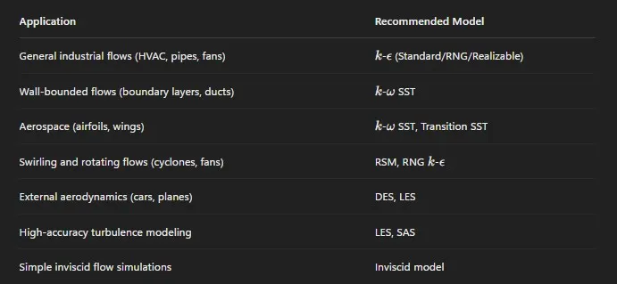
In short,
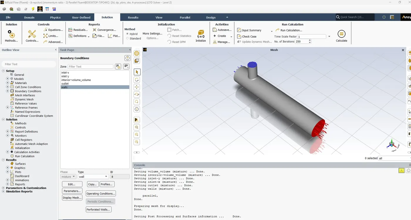
Cell Zones - under volume-volume the material is assigned as air
Boundaries - boundaries and initial condition types are automatically taken by the fluent as we given the names to them.
- Inlet X - velocity: 3 m/s; temperature: 36-degree Celsius
- Inlet Y - velocity: 6 m/s; temperature: 19-degree Celsius
- Outlet - assumed as the gauge pressure (0 Pa)
Initialization:
Standard initialization:
- Assigns uniform values for velocity, pressure, and temperature throughout the domain.
- Uses user-defined inputs or a reference cell.
- Works well for simple cases but may not be accurate for complex flows.
Hybrid initialization:
- Solves a Laplace equation to estimate velocity and pressure distributions.
- Accounts for flow gradients to provide a better initial guess.
- Helps in faster convergence and is useful for complex flows (turbulence, recirculation, etc.).
CASE 1:
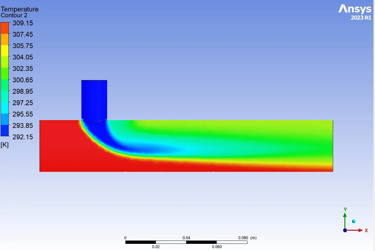
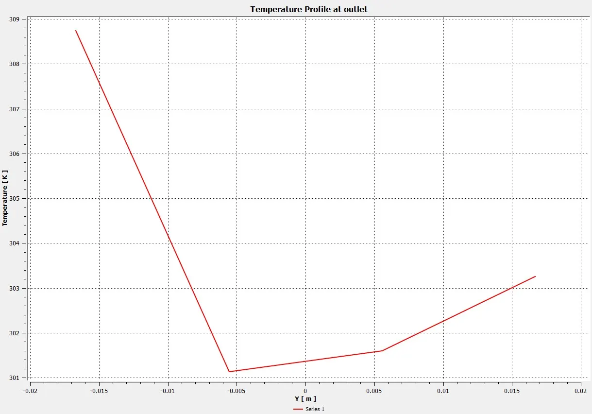
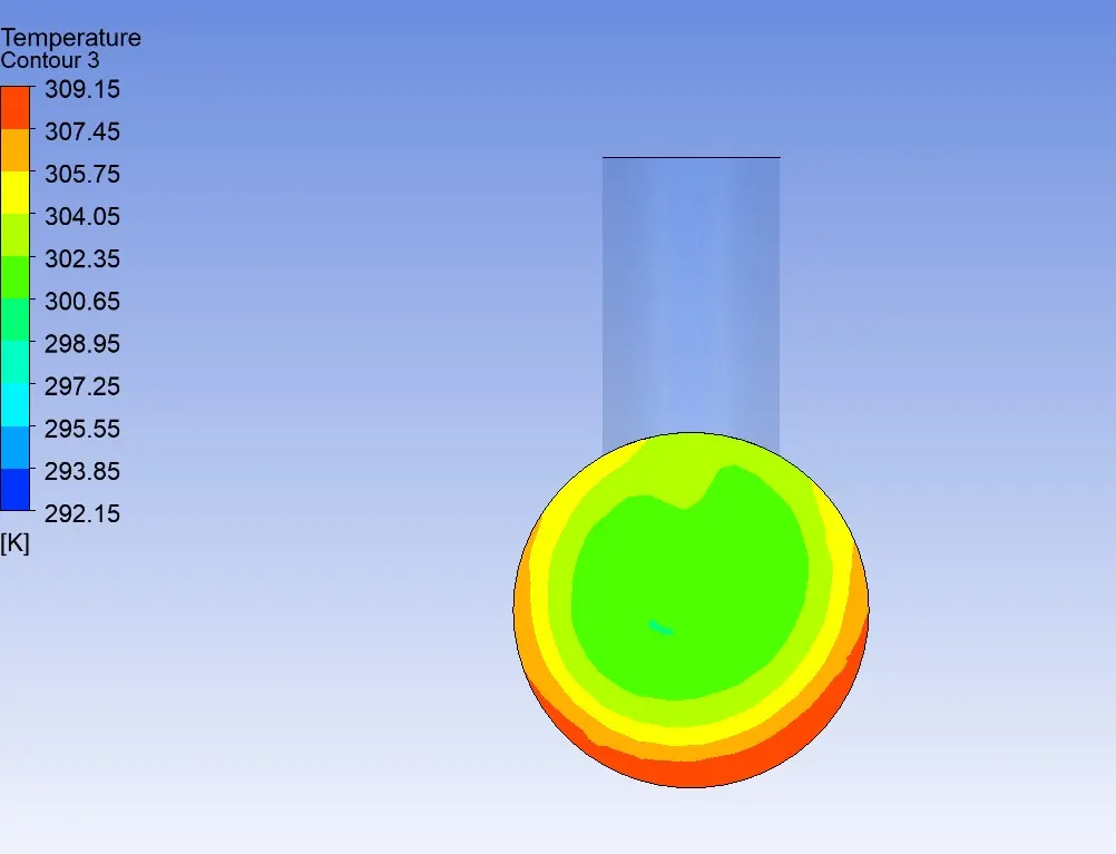
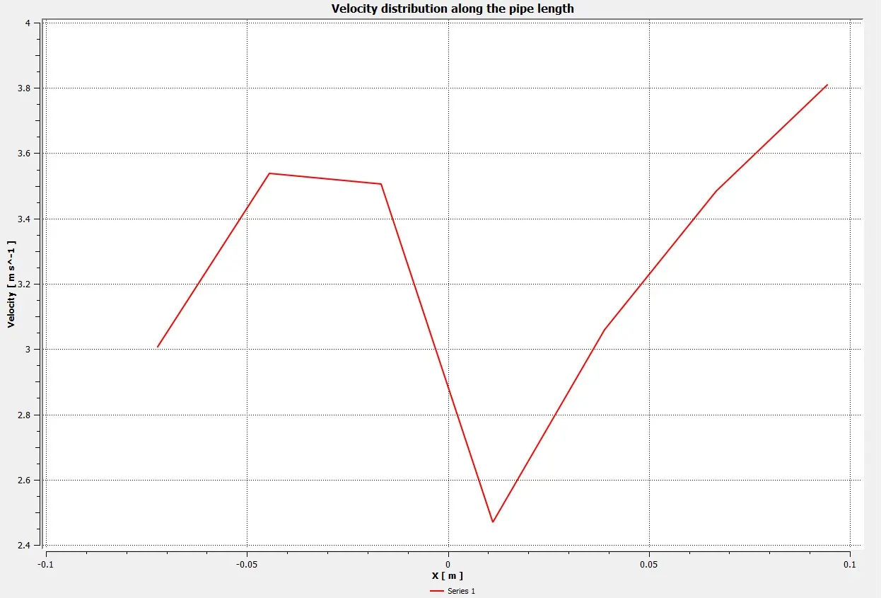
Hot mixing tee with an inlet velocity of 3 m/s its corresponding temperature is 36-degree Celsius and outlet velocity is 6 m/s its corresponding temperature is 19-degree Celsius.
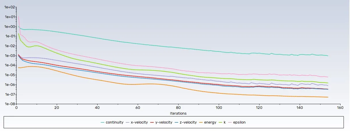
Viscous model (k-epsilon STANDARD)
Scaled residuals:
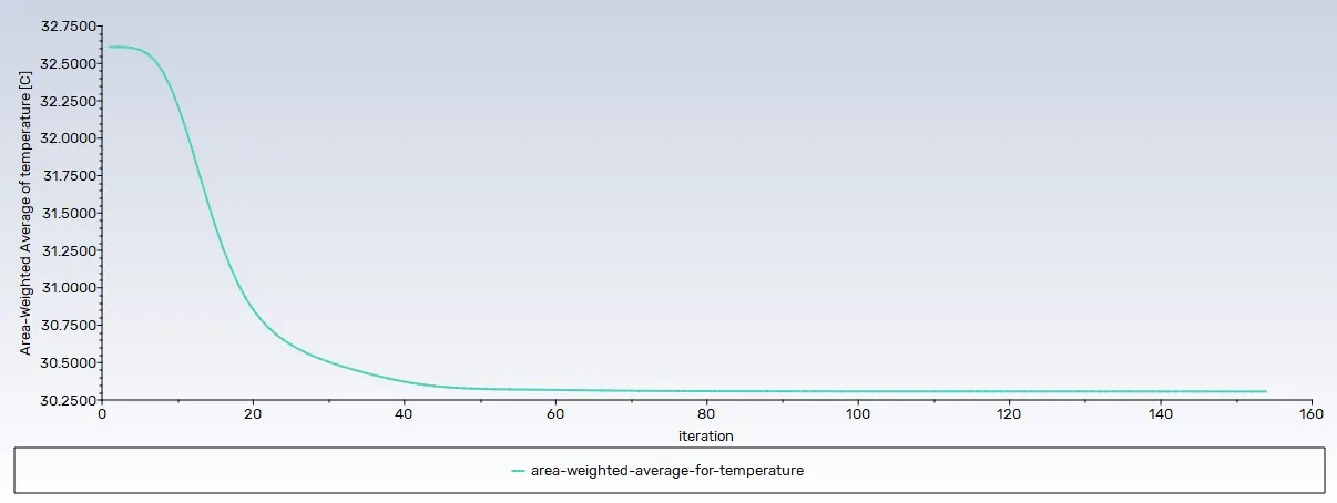
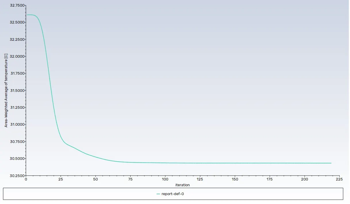
Area weighted average for temperature:
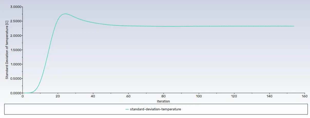
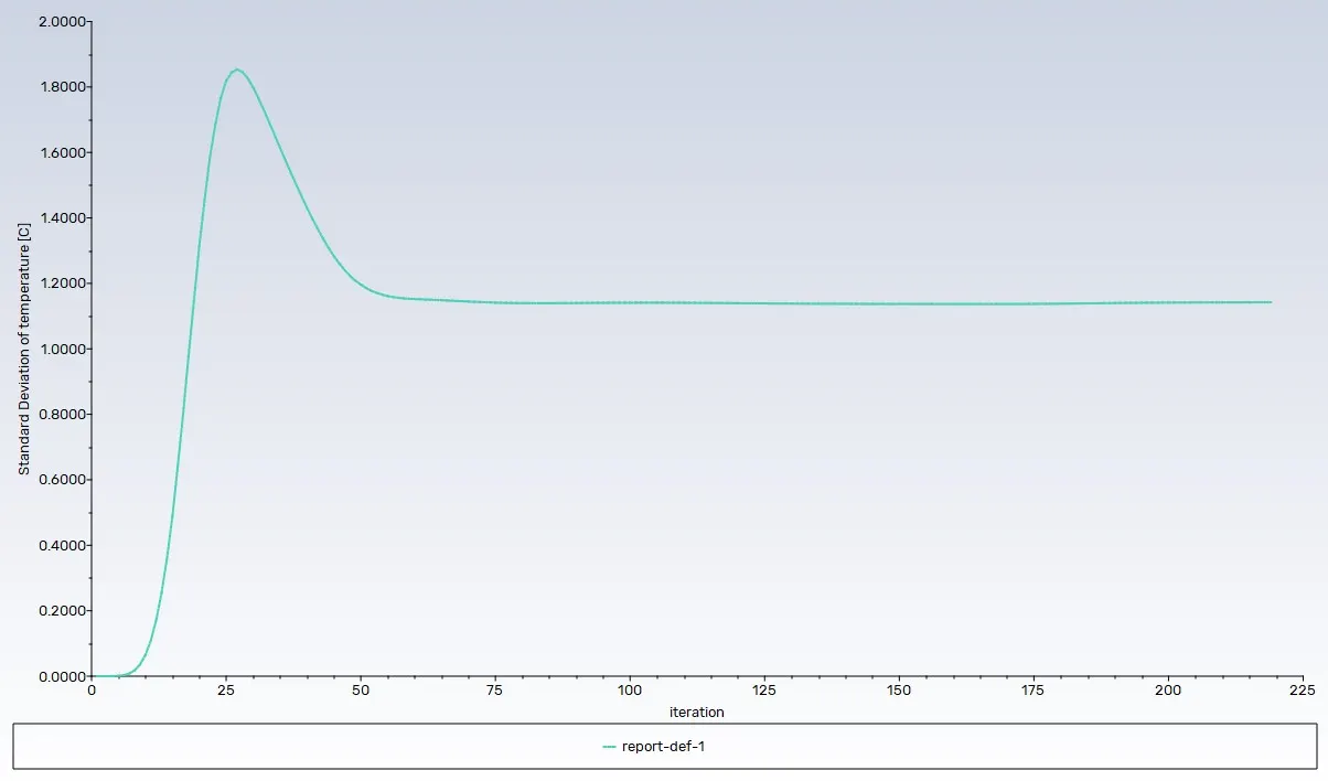
Standard deviation for temperature:
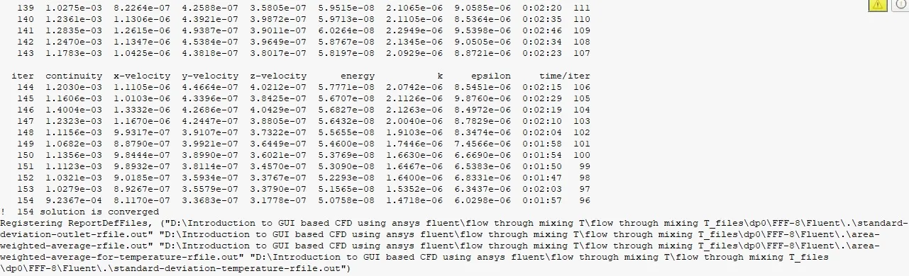
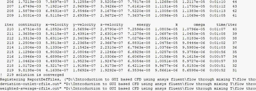
Convergence:
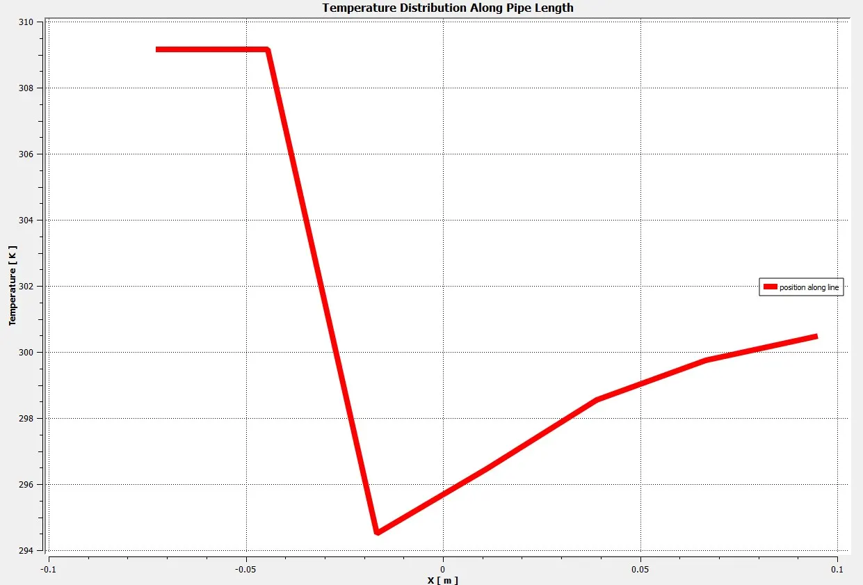
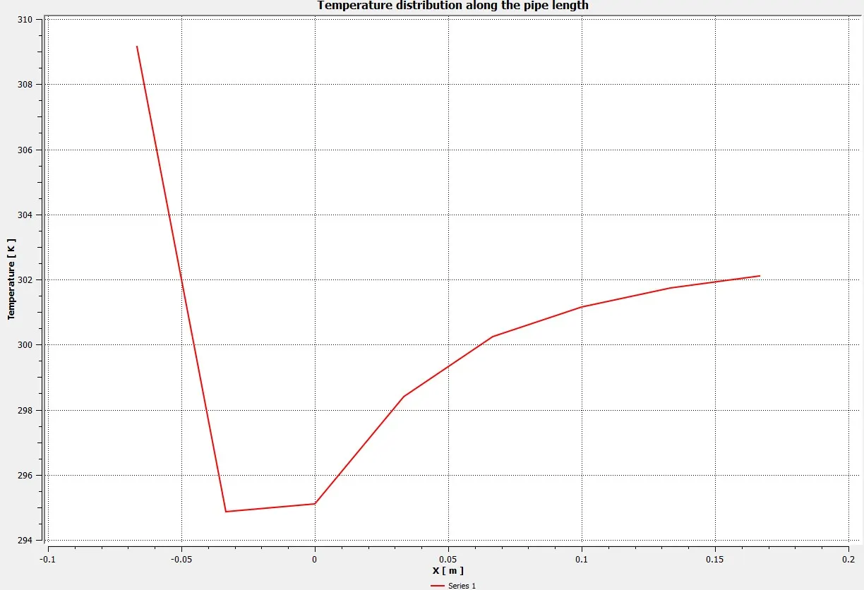
Temperature distribution along the pipe length:
Temperature Profile at outlet:
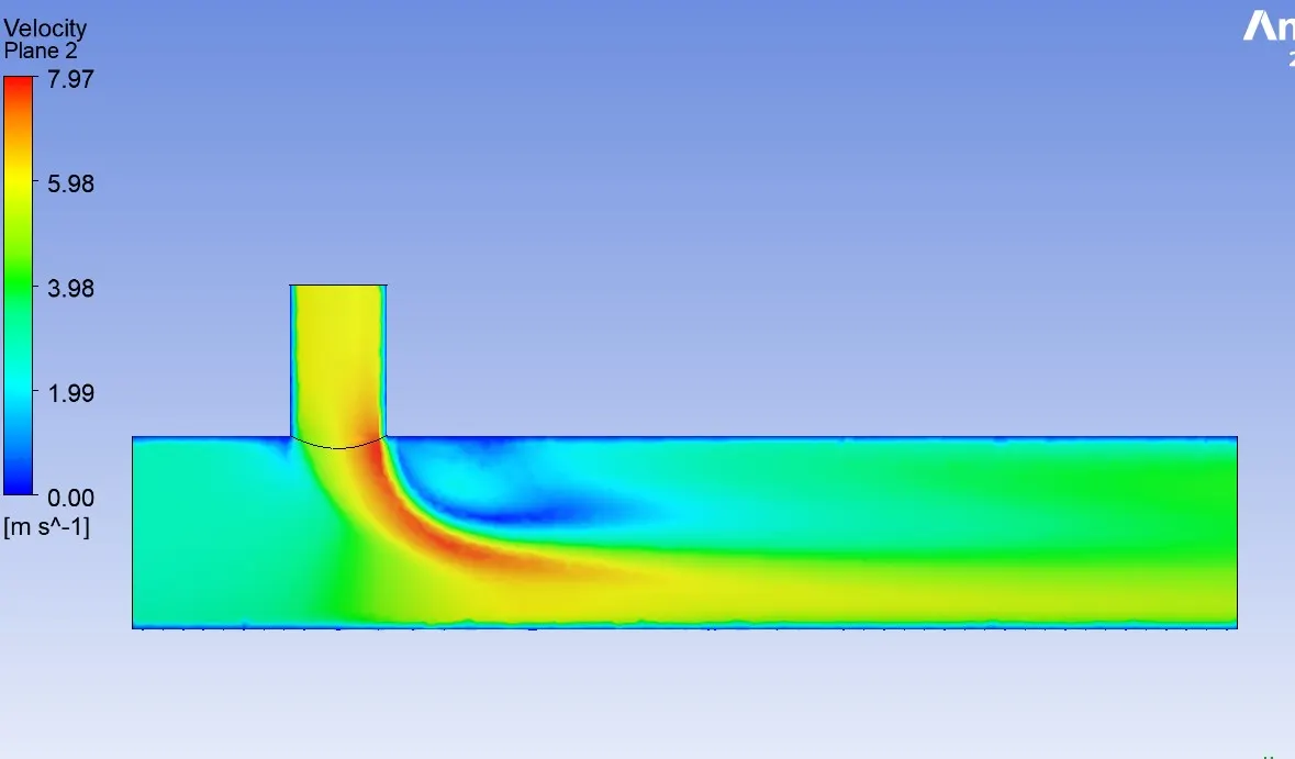
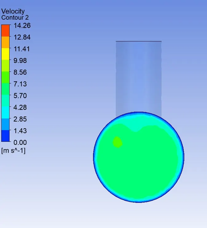
Velocity distribution along the pipe length:
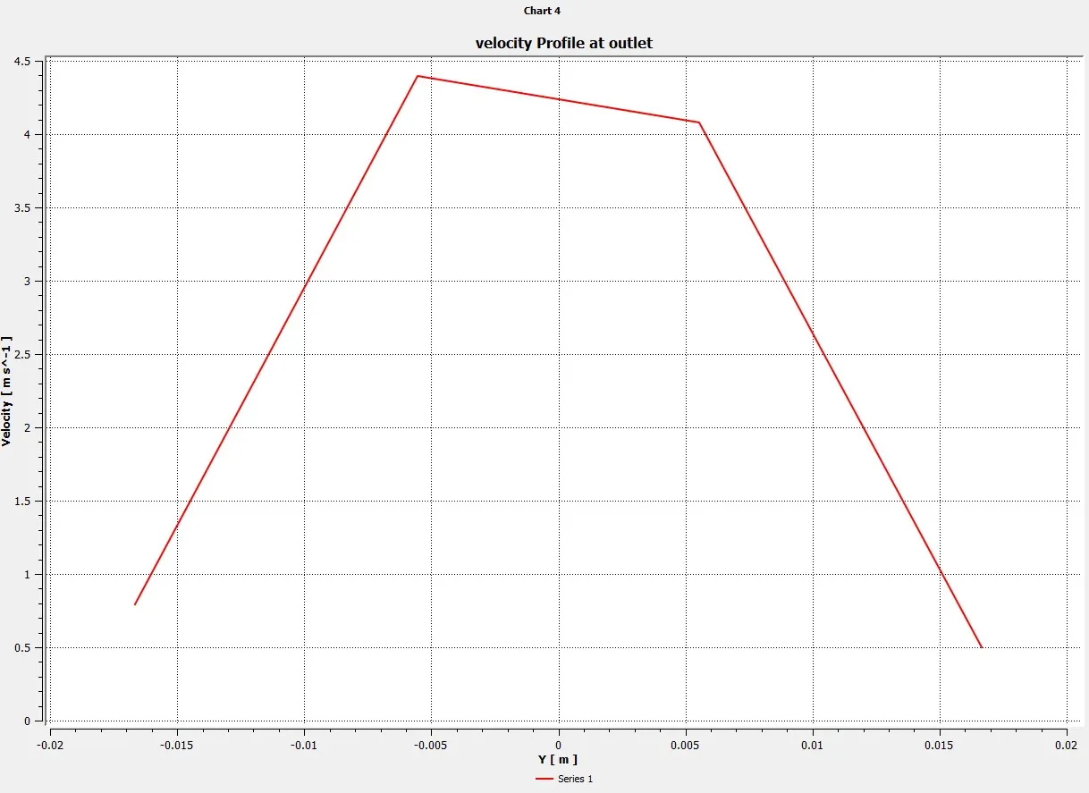
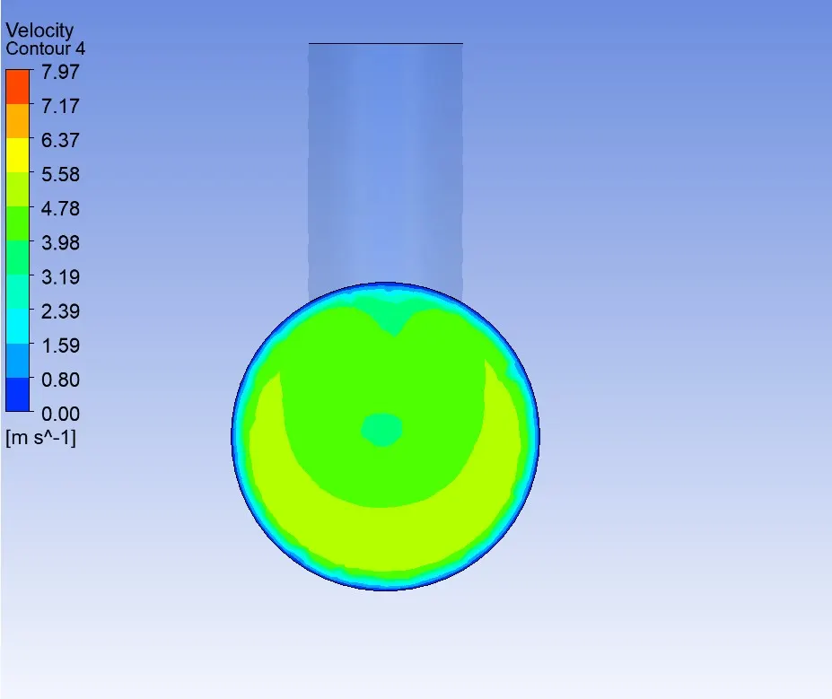
velocity Profile at outlet:
CASE 1:
Hot mixing tee with an inlet velocity of 3 m/s its corresponding temperature is 36-degree Celsius and outlet velocity is 6 m/s its corresponding temperature is 19-degree Celsius.
Viscous model (k-omega SST)
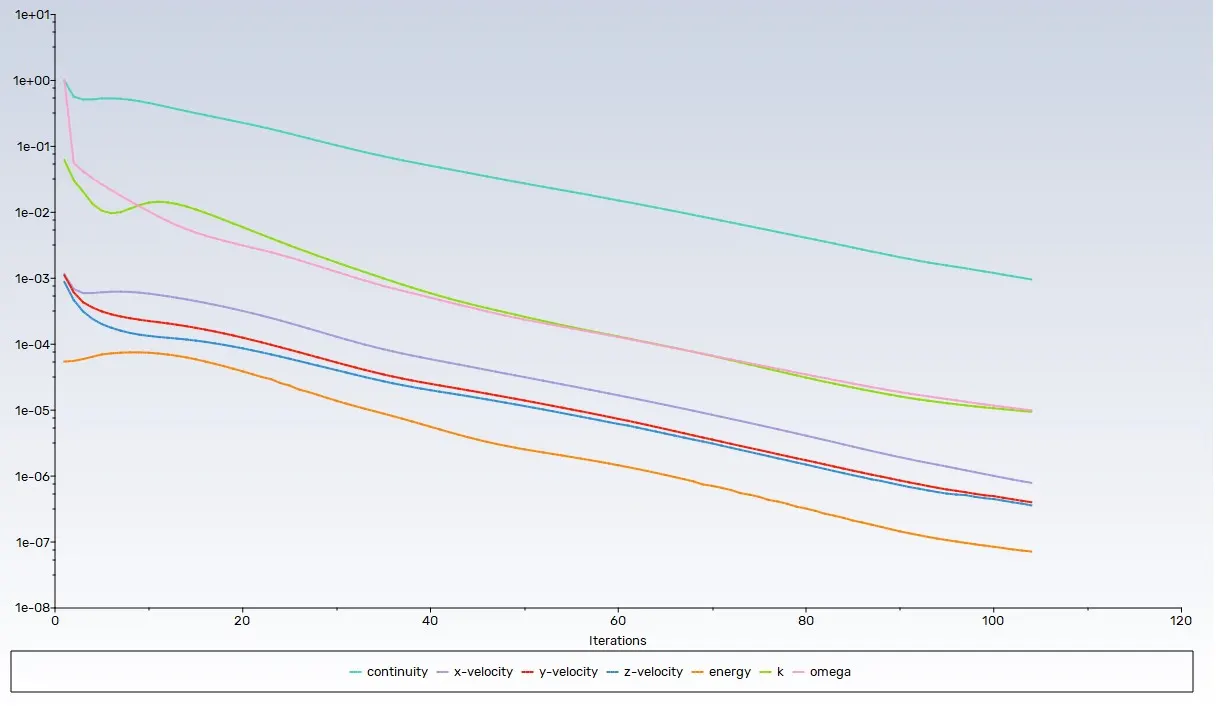
Scaled residuals:
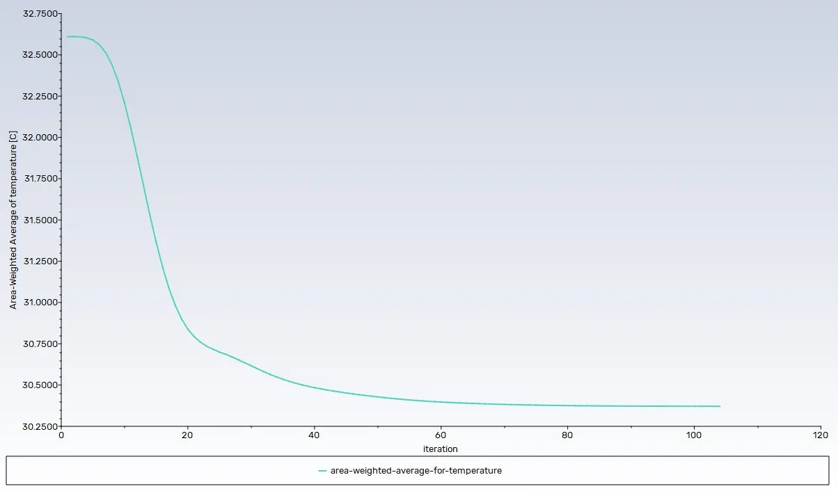
Area weighted average for temperature:
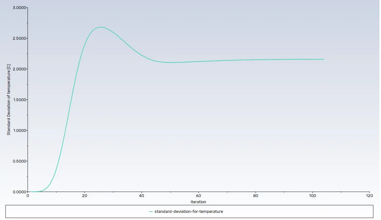
Standard deviation for temperature:
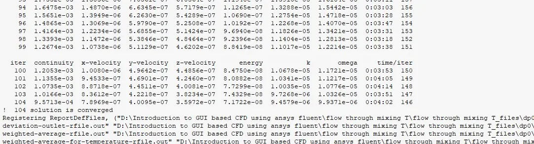
Convergence:
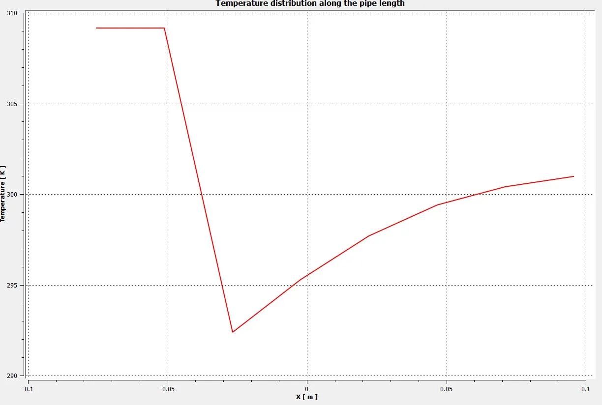
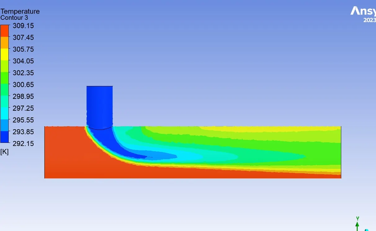
Temperature distribution along the pipe length:
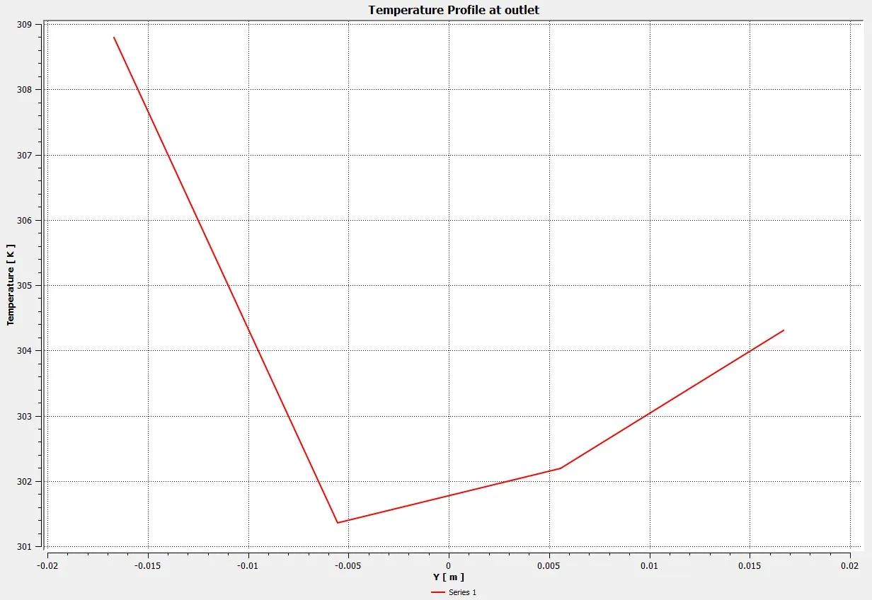
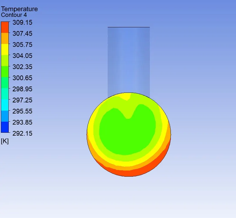
Temperature Profile at outlet:
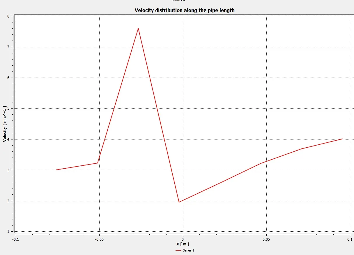
Velocity distribution along the pipe length:
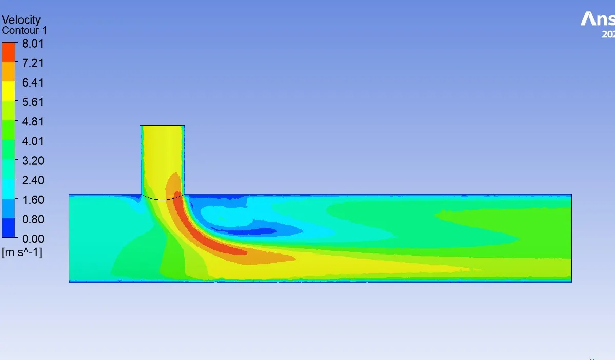
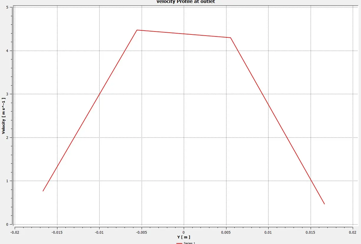
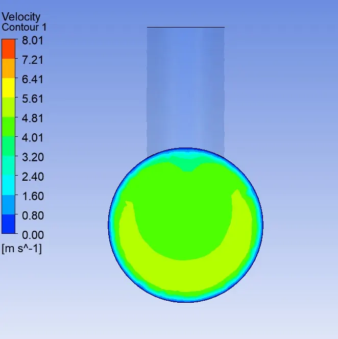
velocity Profile at outlet:
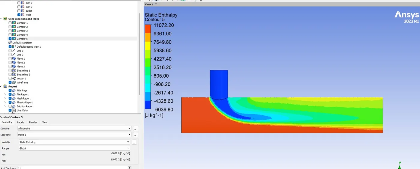
STATIC ENTHALPHY:
Comparison of k-epsilon STANDARD and K-omega SST:
Velocity contour comparison:
K-epsilon STANDARD:
- predicts a smoother velocity profile but may overestimate turbulence
- fails to accurately capture recirculation zones in the mixing region
K-omega SST:
- show sharper velocity gradients and better near wall effects
- accurately predicts flow separation and reattachment at the junctions
Temperature contour comparison
K-epsilon STANDARD:
- predicts more uniform temperature distribution but lacks bear wall accuracy.
- misses localized thermal gradients in high shear regions
K-omega SST:
- provides better temperature resolution near walls and mixing regions
- captures thermal stratification and temperature fluctuations more accurately
for the above comparison, K-omega SST achieved convergence in fewer iteration because it captured velocity and temperature gradient more efficiently. Hence for further analysis we will move forward with K-omega SST viscous method.
CASE 1:
Hot mixing tee with an inlet velocity of 3 m/s its corresponding temperature is 36-degree Celsius and outlet velocity is 12 m/s its corresponding temperature is 19-degree Celsius.
Viscous model (k-omega SST)
Scaled residuals:
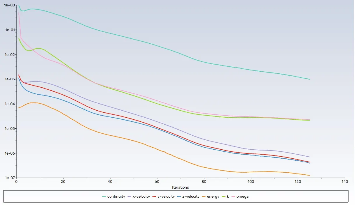
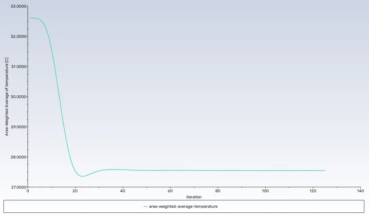
Area weighted average for temperature:
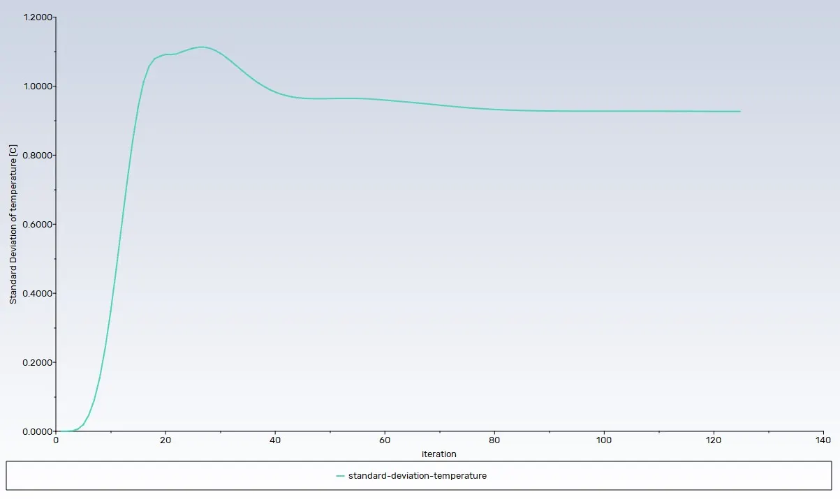
Standard deviation for temperature:
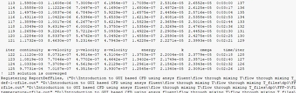
Convergence:
Temperature distribution along the pipe length:
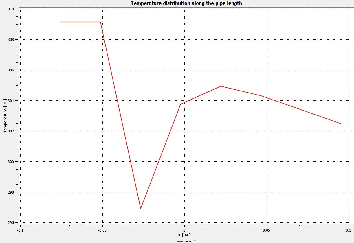
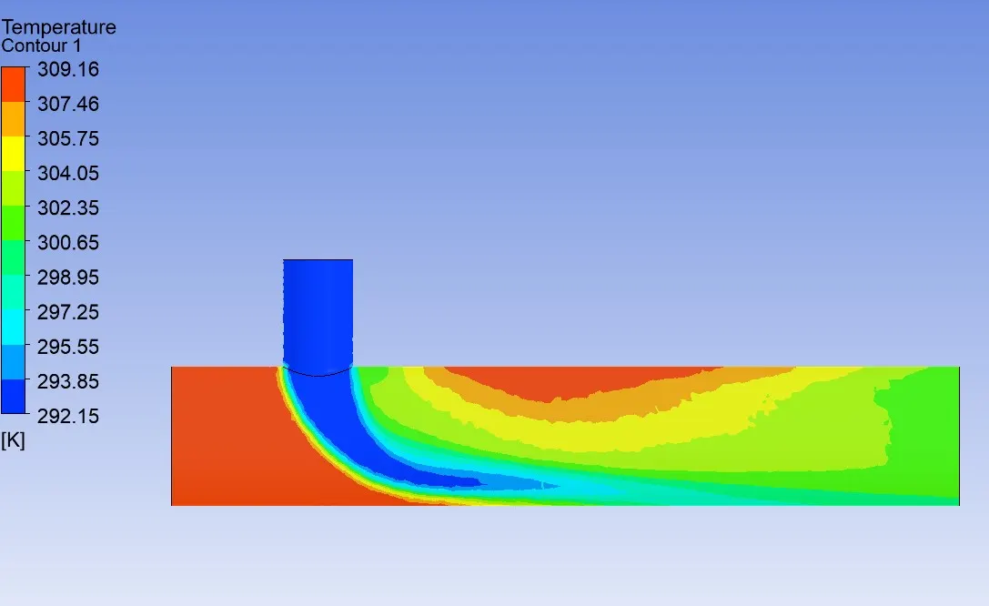
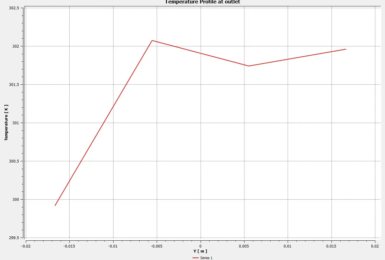
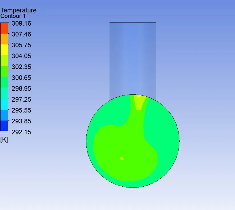
Temperature Profile at outlet:
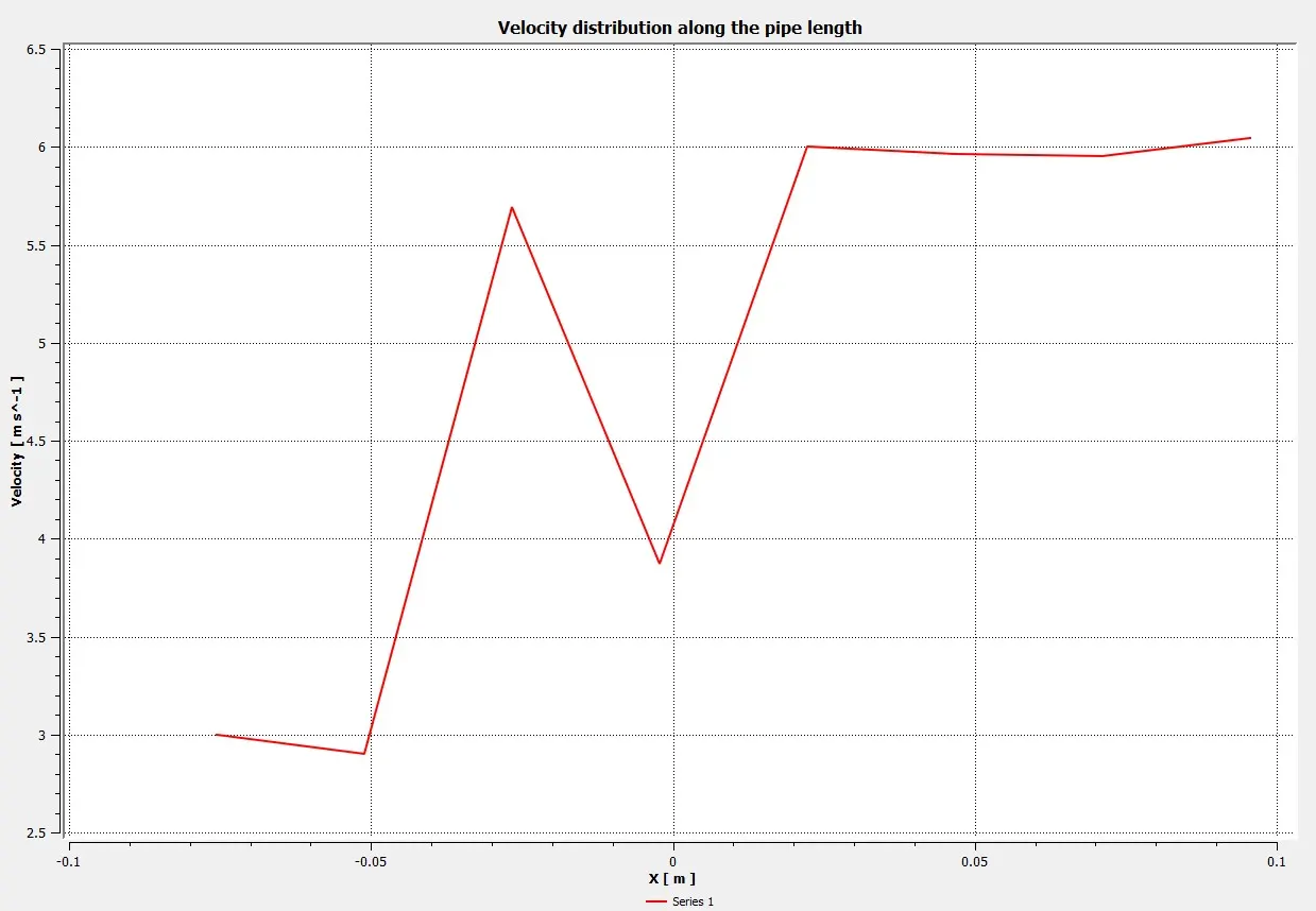
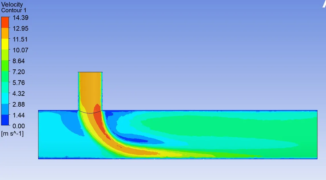
Velocity distribution along the pipe length:
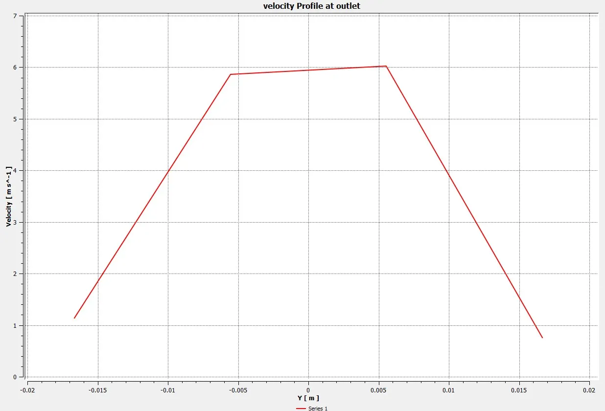
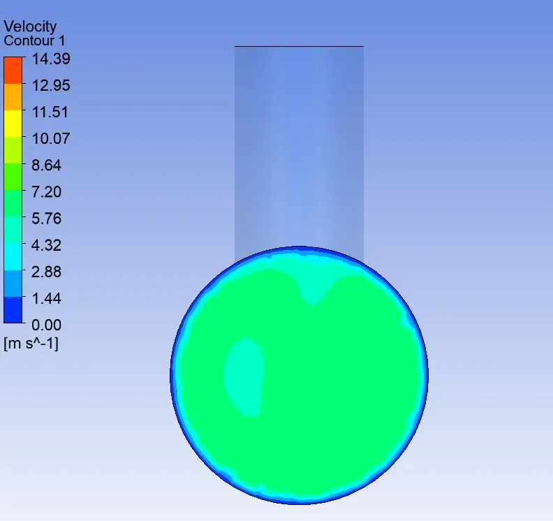
velocity Profile at outlet:
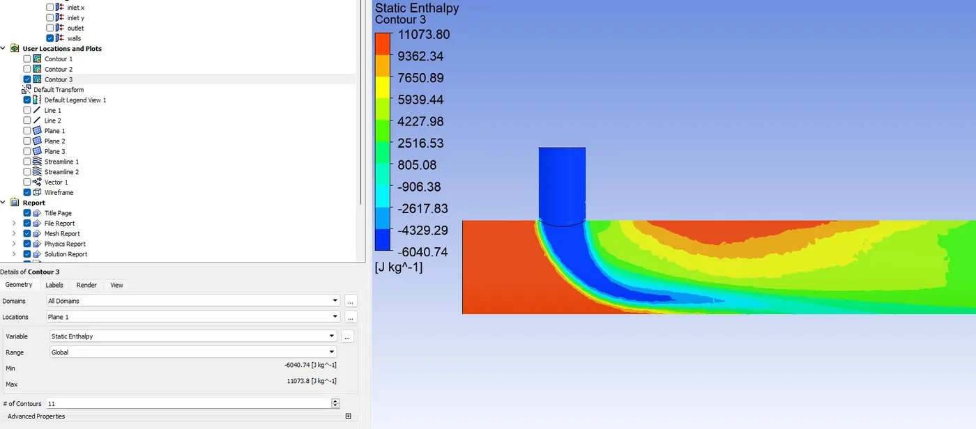
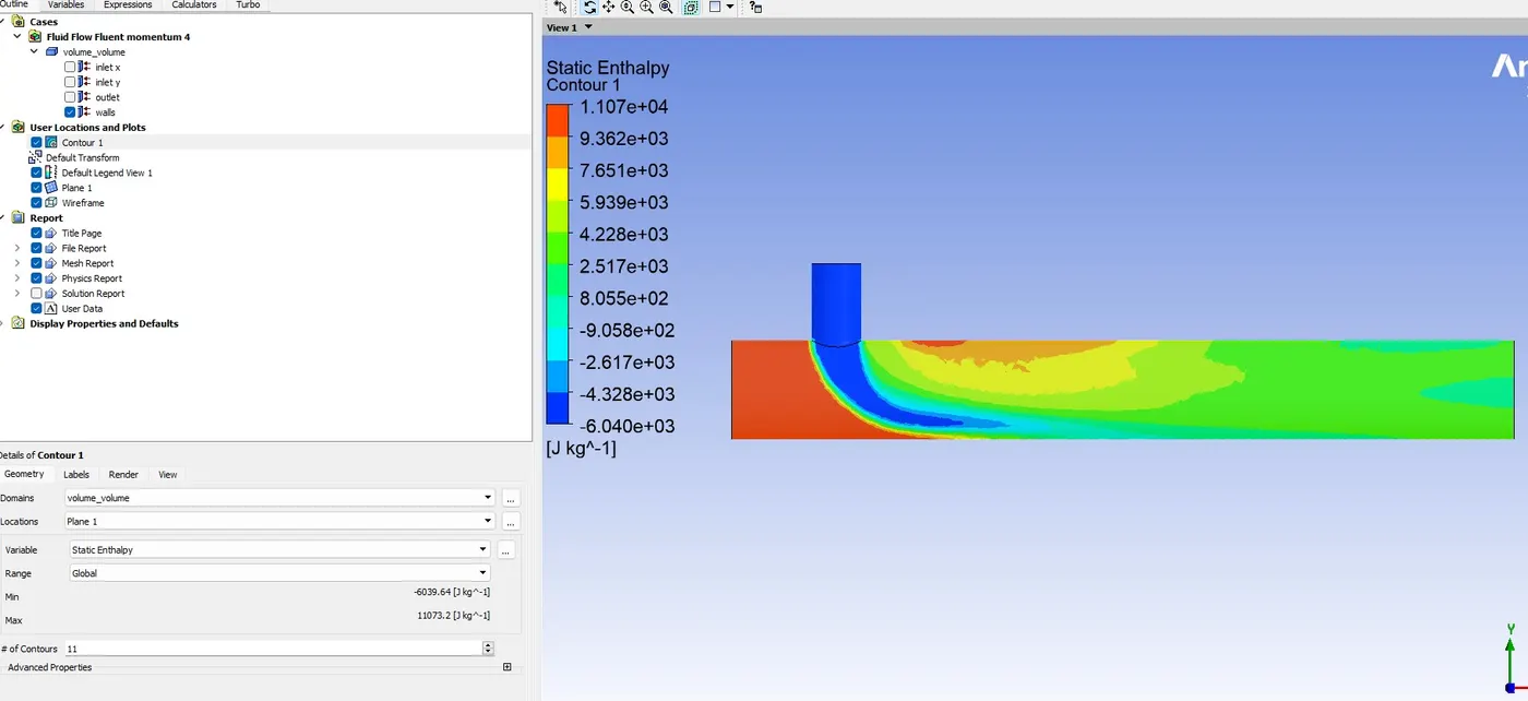
STATIC ENTHALPHY:
CASE 2:
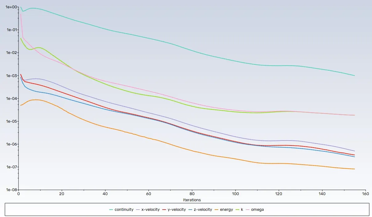
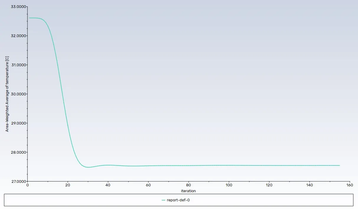
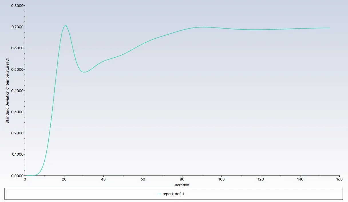
Hot mixing tee with an inlet velocity of 3 m/s its corresponding temperature is 36-degree Celsius and outlet velocity is 12 m/s its corresponding temperature is 19-degree Celsius.
Viscous model (k-omega SST)
Scaled residuals:
Area weighted average for temperature:
Standard deviation for temperature:
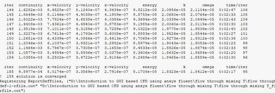
Convergence:
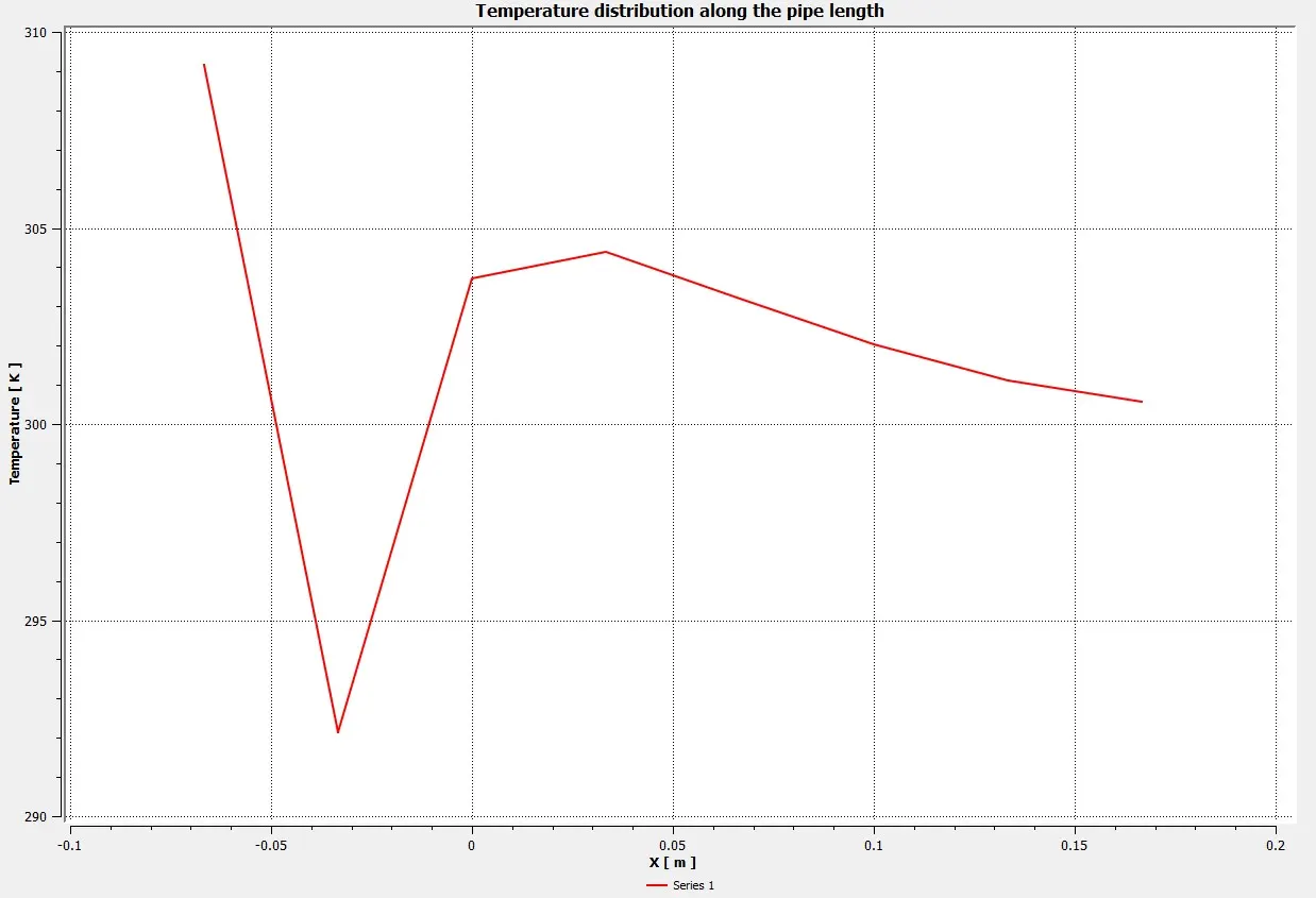
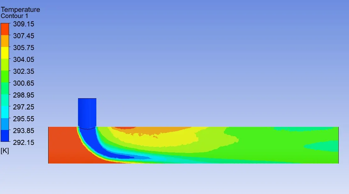
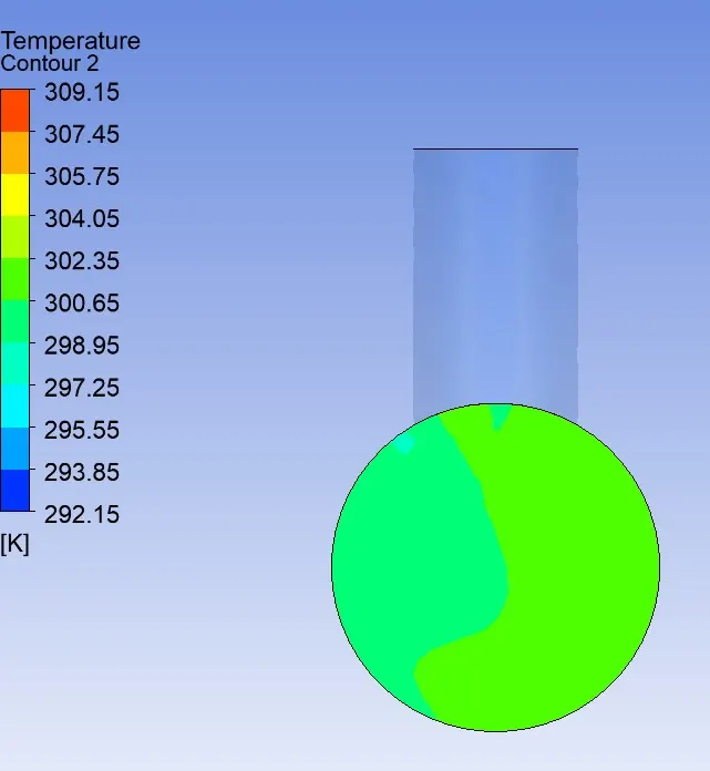
Temperature distribution along the pipe length:
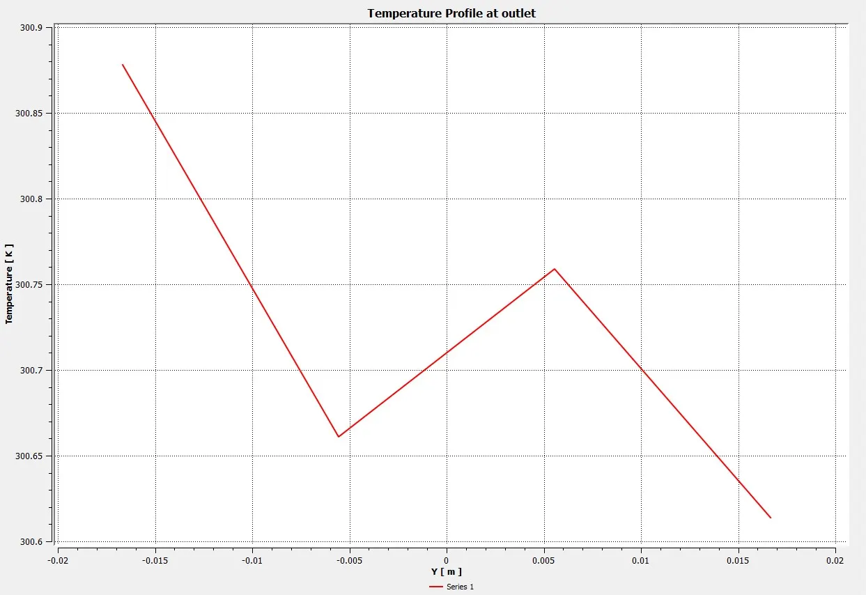
Temperature Profile at outlet:
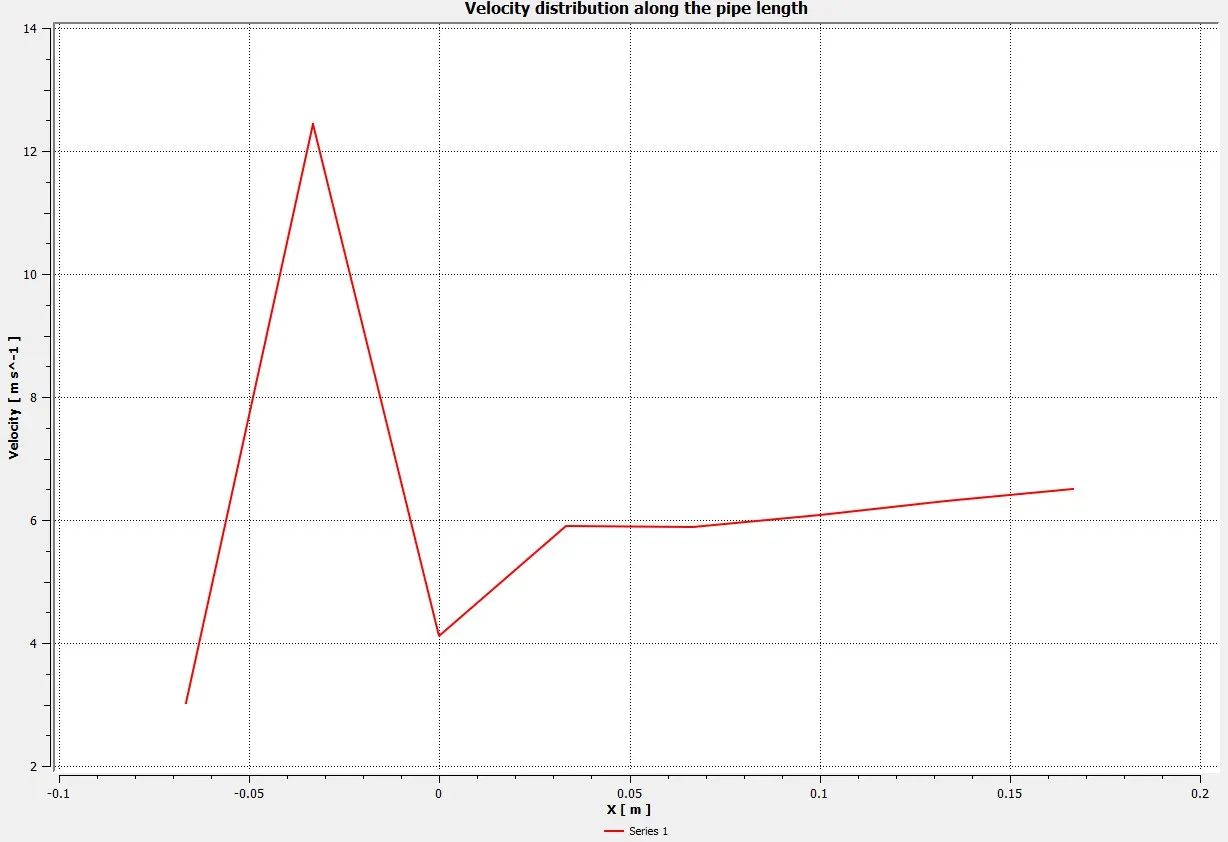
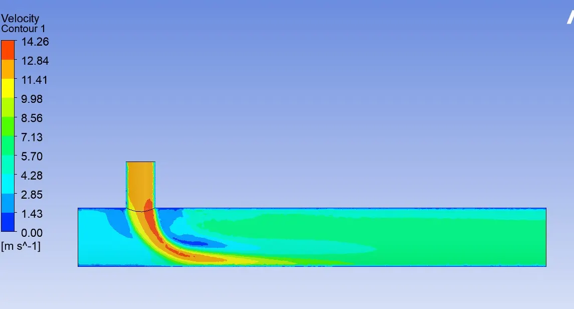
Velocity distribution along the pipe length:
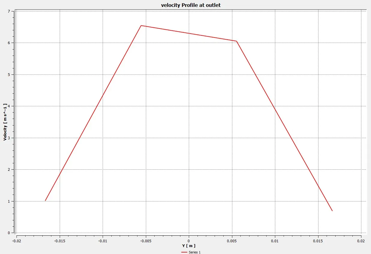
velocity Profile at outlet:
STATIC ENTHALPHY:
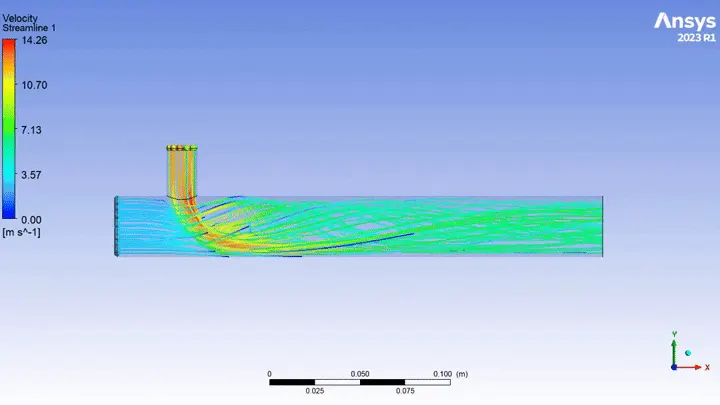
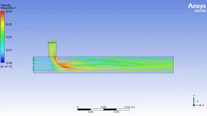
Streamline video:
CASE 2:
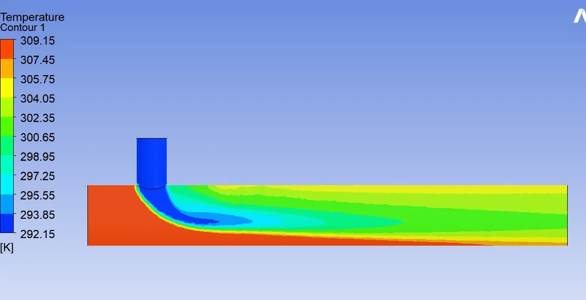
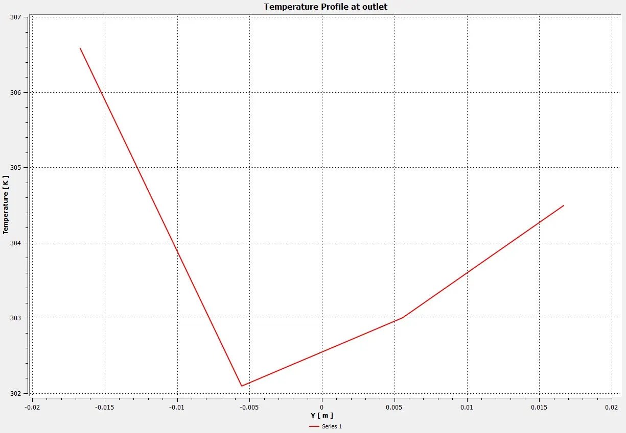
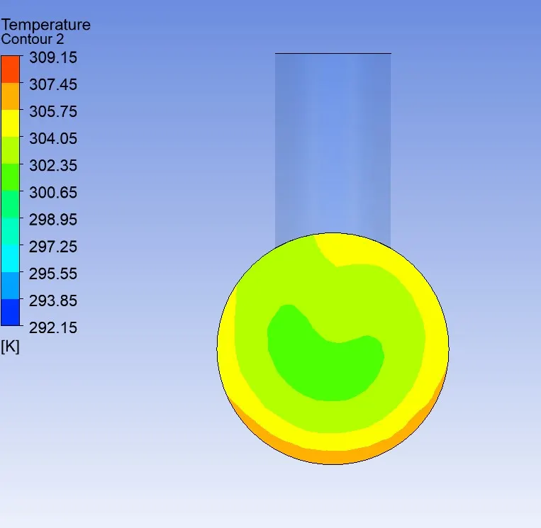
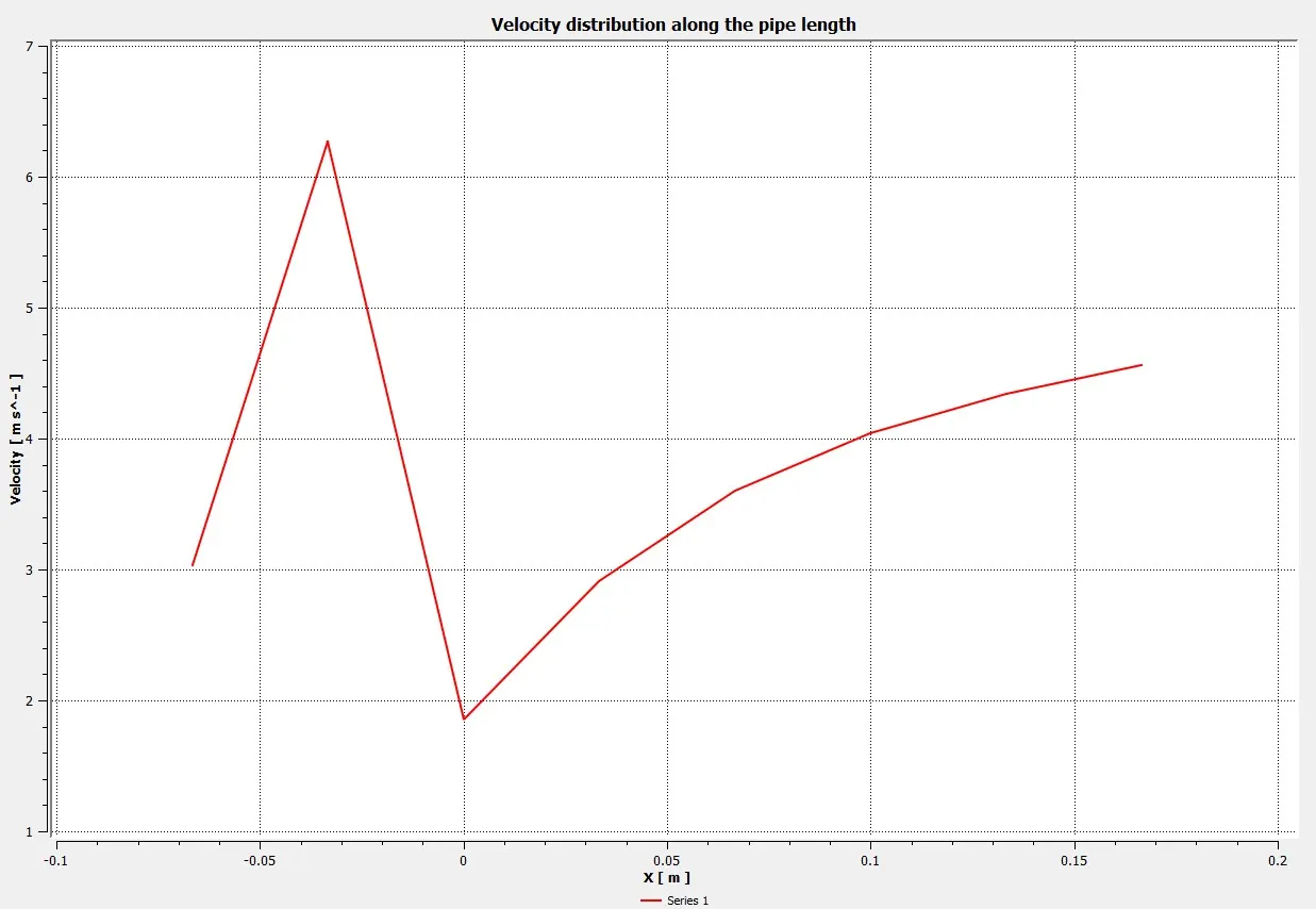
Hot mixing tee with an inlet velocity of 3 m/s its corresponding temperature is 36-degree Celsius and outlet velocity is 6 m/s its corresponding temperature is 19-degree Celsius.
Viscous model (k-omega SST)
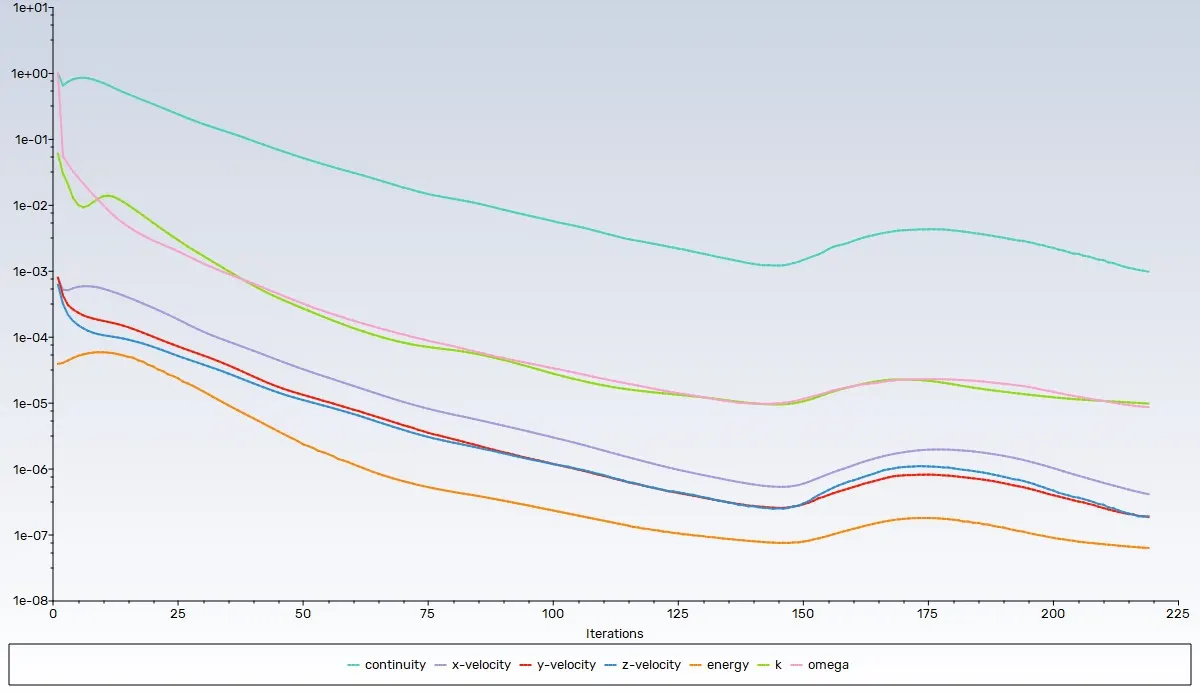
Scaled residuals:
Area weighted average for temperature:
Standard deviation for temperature:
Convergence:
Temperature distribution along the pipe length:
Temperature Profile at outlet:
Velocity distribution along the pipe length:
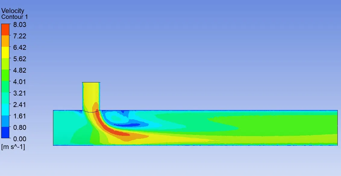
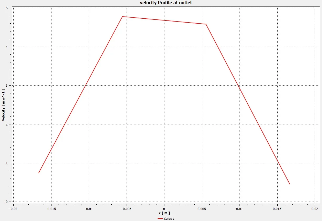
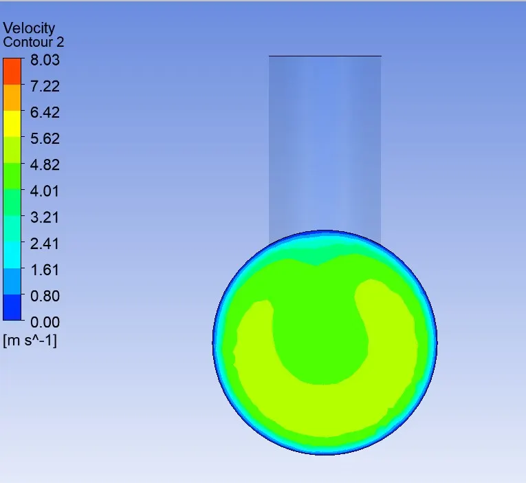
velocity Profile at outlet:
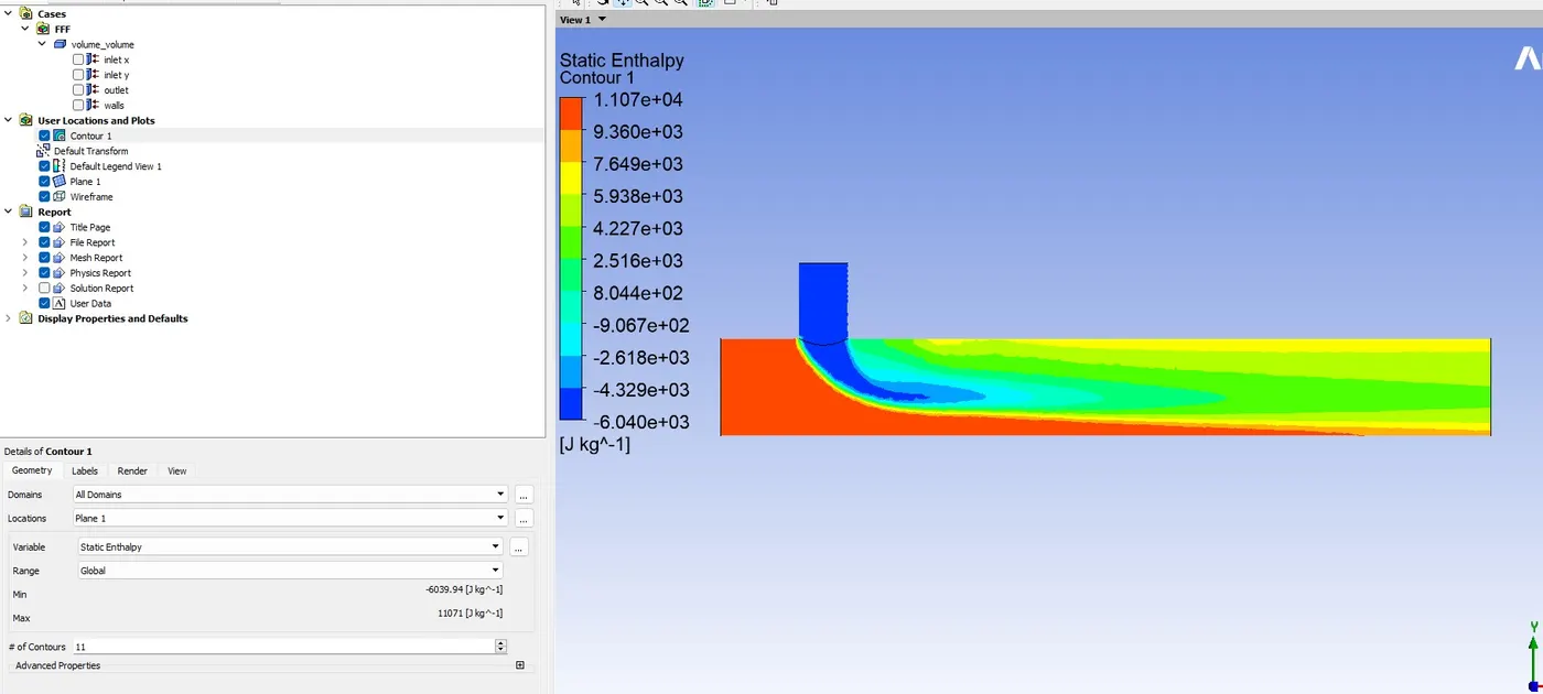
STATIC ENTHALPHY:
Streamline video:
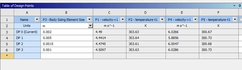
GRID DEPENDENCENY TEST FOR CASE 2: (LONG TEE)
As we can see, the at mesh size 0.002 m, the solution has relatively converged with very minimum deviation, this ensures we are working with hybrid mesh model i.e. with quite good accuracy and less computational cost.
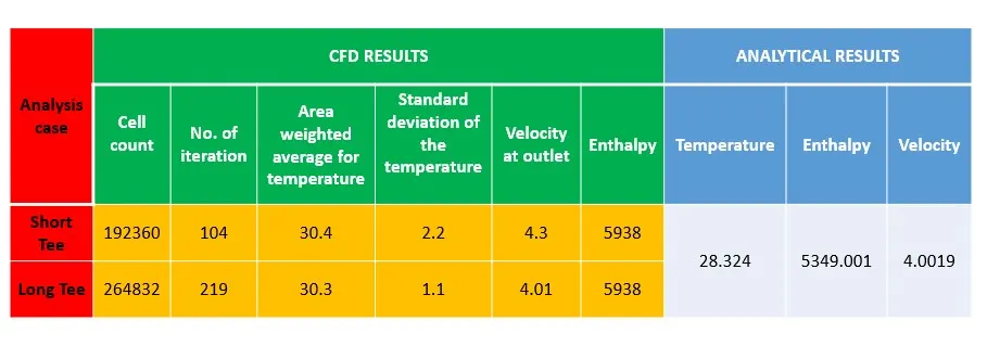
RESULT DISSCUSION:
Hot mixing tee with an inlet velocity of 3 m/s its corresponding temperature is 36-degree Celsius and outlet velocity is 6 m/s its corresponding temperature is 19-degree Celsius.
Viscous model (k-omega SST)
Hot mixing tee with an inlet velocity of 3 m/s its corresponding temperature is 36-degree Celsius and outlet velocity is 12 m/s its corresponding temperature is 19-degree Celsius.
Viscous model (k-omega SST)
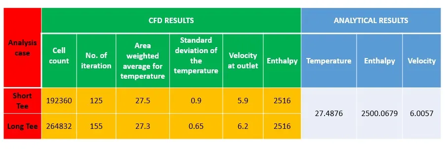
- as we can see that there is much larger standard deviation in the short pipe while compared to long pipe. this is due to the uneven or not a complete mixing in the short pipe while compared to long.
- the result in long pipe is almost close to the analytical results this is because the analytical result is calculated as it has complete mixture, but whereas in long tee, at the outlet we can see that the velocity profile is started growing to laminar. if we increase the pipe further, we can see the results much equal to analytical
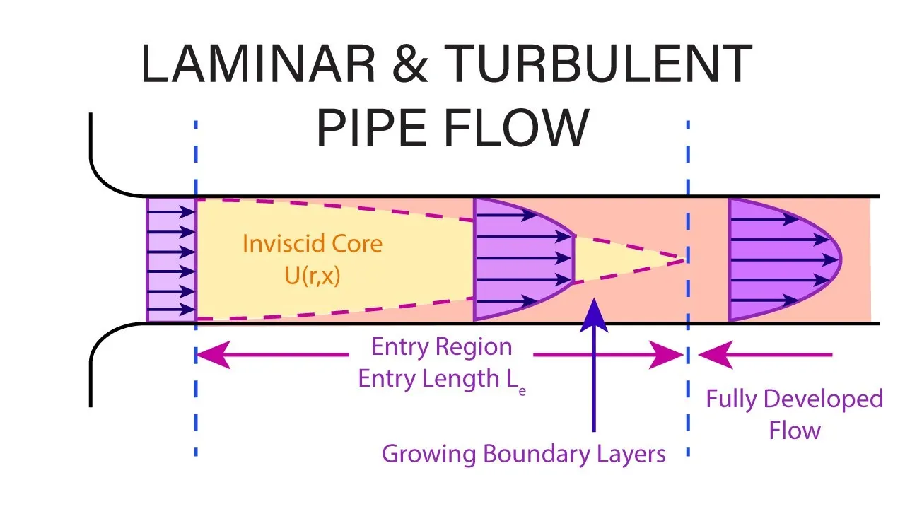
- for a momentum ratio of 2, the fully developed laminar i.e. complete mixture of fluids will be take place at the length of 0.679m
- for a momentum ratio of 4, the fully developed laminar i.e. complete mixture of fluids will be take place at the length of 0.727m
- so, the length of the pipe plays the important role to get the fully developed flow or a complete mixture of the fluids
- and also, we can see that as inlet velocity of the pipe increase, there is a large turbulent formed this provide a better mixing as long pipe
- standard deviation also comparatively small in momentum ratio - 4 with small tee.
- Hence the suggestion is. either we want to increase the velocity flow or increase the length of the pipe to get better mixing
Reference:
https://www.sciencedirect.com/science/article/abs/pii/S0029549309005676?via%3Dihub
File link:
https://drive.google.com/file/d/185Sj1bI6iQy_2f5kDSqw1PUpI8uY6oeo/view?usp=drive_link