Week 1- Mixing Tee

This assignment will be discussed case by case.

For Short Pipe:

1) Momentum Ratio 2:

On opening Ansys workbench, from the toolbox, the project schematic for “Fluid Flow (Fluent)” was selected. The simulation set up starts with opening Discovery. There, the supplied model is opened and inspected. In the “Prepare” tab, the “Volume Extract” tab is selected. This is done so as to exclude the solid shell of the pipe from the steady state simulation as we are only interested in how the fluid inside the pipe is mixing and we are not bothering with heat flow through the pipes. The volume is extracted by selecting the edges of the internal volume. Ansys then encloses this box by an imaginary box. This is what helps the software with meshing.

Once the volume extraction is done, we can see that the tree for the model contains both the extracted volume and the shell. The shell can be excluded from the simulation by clicking on the leftmost icon (next to the “hide” button).

After this, we update our progress in the meshing module from the workbench and initialise the meshing module.

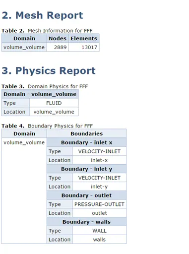
Once the meshing module starts, using the ‘CTRL+F’, the face selection was enabled. The oulet was selected and was accordingly named “Outlet”. Similarly, the “Inlet-Y”, “Inlet-X” and the “Walls” were selected and named. To make multiple selection for the walls, the ‘CTRL’ button was used while selecting the walls enclosing ‘Inlet-Y’ after the walls along the outlet were first selected.

The next step was to mesh the model. On left clicking the ‘Mesh’ option in the tree for the project on the “Outline” window, a mesh was automatically generated.

Next step is to launch ‘Fluent’. This can be done by updating the ‘Set-Up’ in the project schematic on ‘Workbench’ and selecting it. The “Fluent launcher” then opens. The ‘Dimension’ is selected to ‘3D’ and the ‘Double Precision’ option is selected.

In the ‘Mesh’ group in the ‘Domain’ tab, the option for checking the mesh is used. Once the Console puts out the message saying that the checks are done without issuing any warnings, we then set-up the solver.

The type of the solver is set to “Pressure-based”, velocity formulation to “Absolute” and since we are attempting to run a steady state simulation, we check the option to “Steady”.

Then, we move on to the ‘Physics’ tab and in the ‘Models’ group, the ‘Energy’ option is checked. This is because we are including temperature also as a variable in this simulation.

Then from the ‘Viscous’ option, the k-Epsilon (realisable) turbulence model is selected.

In ‘Zones’ tab, we define the boundary conditions in the ‘Boundaries’ option.

For Inlet-X: this is where the warmer air enters. In the momentum tab, the velocity is set to be 3m/s. The reference frame is set to ‘Absolute’ and the ‘Velocity Specification Method’ is set to ‘Magnitude, Normal to the Boundary’. The gauge pressure is set to 0 pascals.

In the ‘Thermal’ tab, the temperature is defined to be 36 degrees Celsius.

For Inlet-Y: this is where the cooler air enters to mix with the warmer air. In the momentum tab, the velocity is set to be 6m/s. The reference frame is set to ‘Absolute’ and the ‘Velocity Specification Method’ is set to ‘Magnitude, Normal to the Boundary’. The gauge pressure is set to 0 pascals.

In the ‘Thermal’ tab, the temperature is defined to be 19 degrees Celsius.

For Outlet: this is where the mixed air exits the pipe volume. It is checked that the guage pressure is set to 0 pascals.

Then we move on to the ‘Solutions’ tab and in the ‘Reports’ group, under ‘Definitions’, the ‘New’ option is clicked to define a new report.

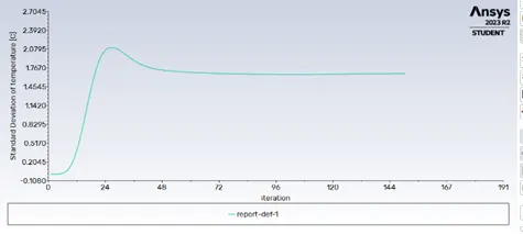
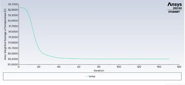
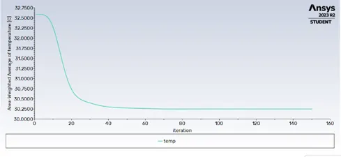
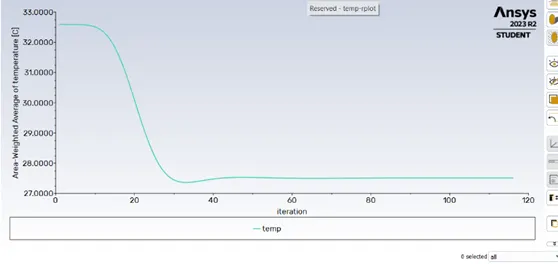
The report for area weighted average of and the report for standard deviation, both of temperatures at the outlet is defined. The Standard Deviation is a good measure for the effectiveness of mixing.

Then the solution is initialised using the ‘Model’.

In the ‘Run Calculation’ tab the ‘Time Scale Factor’ is set to 1 and 150 is inputted for the number of iterations.

Then the calculations are run and after the graphs are obtained, the results are ready for post processing.

The ‘Results’ tab is then opened in the project schematic to initialise ‘CFD-Post’.

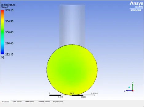
Two planes are inserted, one made along the length of the pipe and one made across the outlet to study the variations in temperatures.

This lets us study the effectiveness of the mixing.

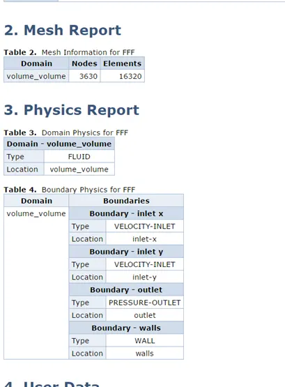
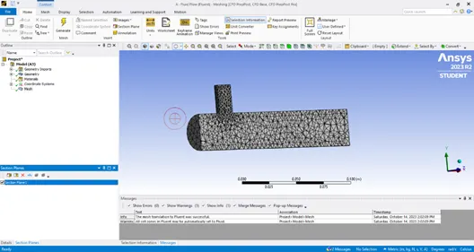(Observing the meshing in the meshing module with the help of a section plane defined across the pipe)

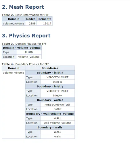
(mesh metric)

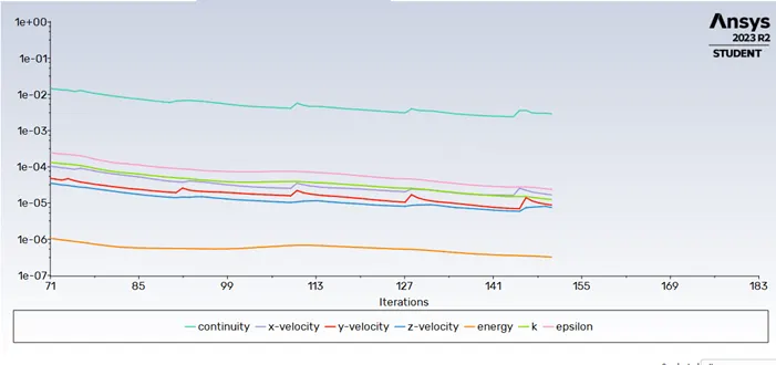
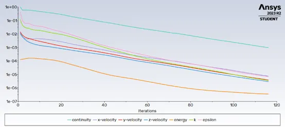
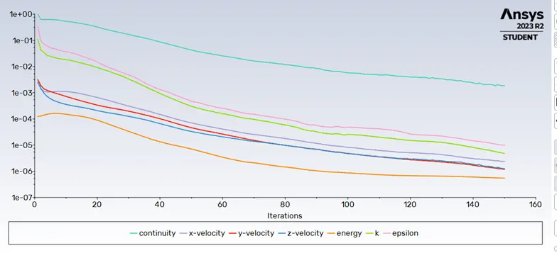
(convergence plot using the k-epsilon turbulence model)

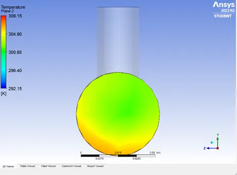
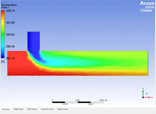
This process of setting up the simulation, but using the k-Omega SST model to compare their convergence plots.

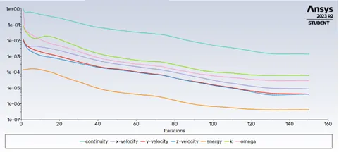
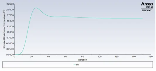
A comparison of the convergence plots (Scaled Residuals vs Iterations) shows that the k-Epsilon model is better suited for this kind of steady state simulations. The residuals are smaller in the case of the k-Epsilon model implying better accuracy. The difference however is difficult to discern. Both could give satisfactory approximations.

The k-Epsilon (realisable) will henceforth be used for all remaining simulations.

1) Momentum Ratio 4:

The above simulation set-up remains the same but the velocity at ‘Inlet-Y’ is set at 12m/s.

The effectiveness of mixing is then to be compared with the previous case.

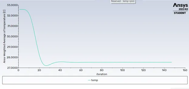
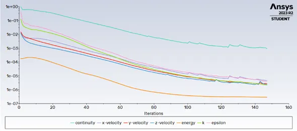
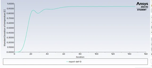
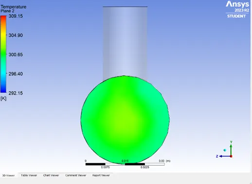
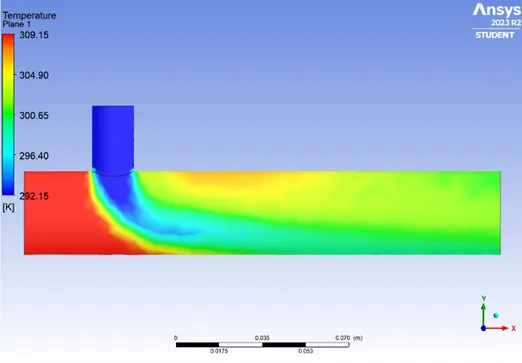
From the data is very clear that the air is now cooler (from the area weighted temperature average plot).

However, the standard deviation of temperature at the outlet is a good measure of mixing effectiveness.

The standard deviation with momentum ratio 4 is lesser than that for ratio 2.

This can also be easily visualised by the temperature gradient on the plane across the outlet.

We can conclude that the air at the outlet is cooler and is better mixed with the increase in velocity at ‘Inlet-Y’

For Long Pipe:

The effect of the increase in velocity (consequently, the momentum ratio) is visible. The effect in the change of length in the mixing effectiveness is now to be studied using the same steady state simulation set-up.

The set up is the same as before but using the model of a longer pipe instead.

1)Momentum ratio 2:

These results were compared with the equivalent one for the short pipe so as to study the effect of length on the mixing effectiveness.

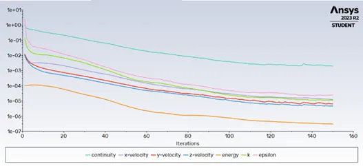
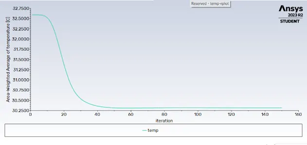
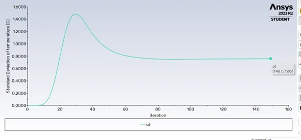
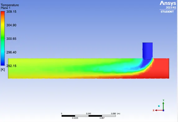
From the graphs it is clear that the area weighted average for the temperature ta the outlet is largely the same. However, the standard deviation plots show a difference. The standard deviation is less for the longer tube (around 0.75) as compared to the compared to the standard deviation for the longer tube (around 1.625). The mixing effectiveness is actually better due to the longer length of the pipe even though the average temperature at the outlet is more or less the same.

This also visible from the temperature gradients. The one for the longer tube is more even, and hence the better mixing is visible to the naked eye.

2)Momentum ratio 4:

The velocity at the Inlet-Y is changed to 12m/s.

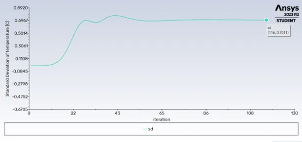
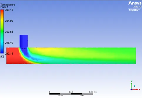
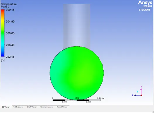
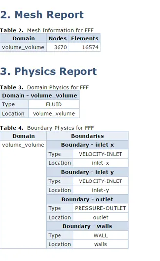
The standard deviation is even lower as compared to the case of the longer pipe with less momentum ratio. The expected trends so far observed is that with increase in inlet velocity (at ‘Inlet-Y), the mixing effectiveness increases as well as the average temperature decreases at the outlet,

This is also visible here. As the inlet velocity was increased, from the graphs, it is visible that the area weighted average of the temperature reduced significantly.

On comparison with the short pipe with moment ratio 4, we see that the standard deviation of temperature at the outlet is lower (somewhere around 0.7 as compared to the neighbourhood of 0.9 for the shorter pipe). This satisfies the expected trend of increase in mixing effectiveness with the length. However, the change in the average temperature at the outlet is not considerable.

From these comparisons drawn from the data collected from my simulations I can conclude that:

1} With increase in length, the standard deviation of temperature at the outlet decreases (implying that the effectiveness of mixing increases), the area weighted average of the temperature at the outlet is almost the same.

2} With increase in momentum ratio, the standard deviation of temperature at the outlet decreases) implying that the effectiveness of mixing increases), the area weighted average of the temperature at the outlet reduces considerably.

Now, to study the effects of a finer mesh the previous case has been repeated with an element size of 0.005.

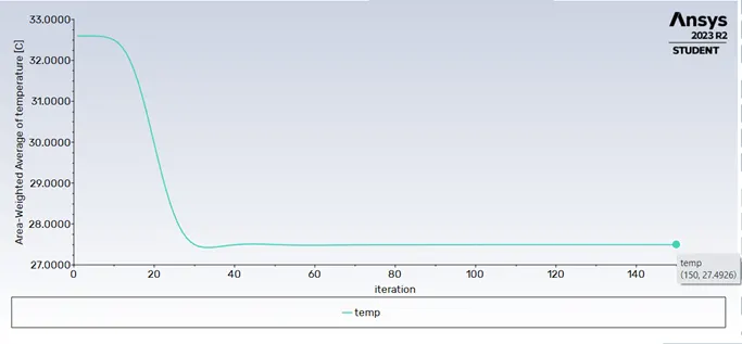
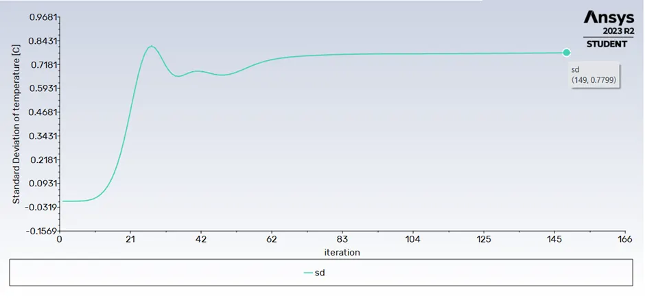
The standard deviation increased 0.7011 for the finer mesh to 0.7799 to the coarser one.

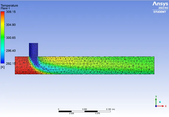(Coarser)

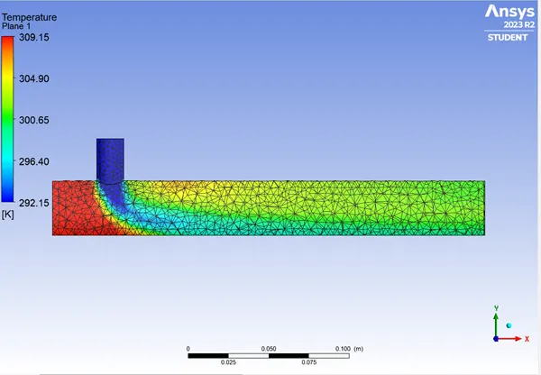(Finer)

Now, the mesh was made even finer, with element size 0.001.

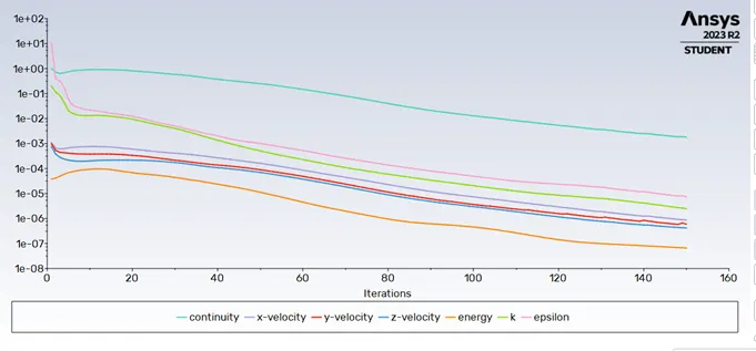
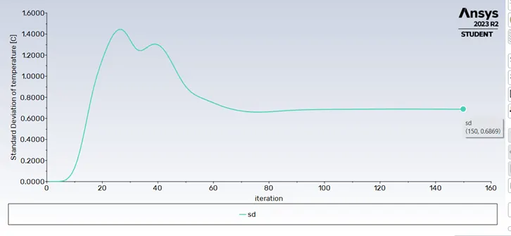
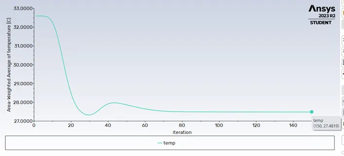
All three cases, seem to be converging to the same answer for area weighted average of the temperature, some where in the neighbourhood of 27.5 degrees celcius.

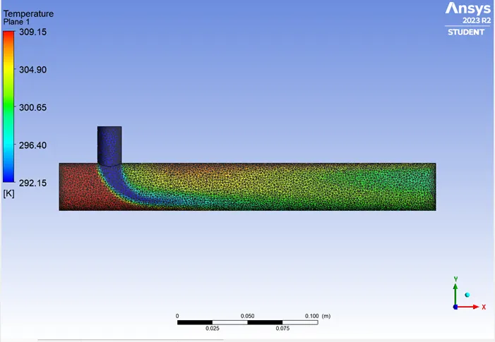
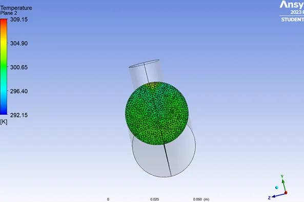
Obviously. The finer mesh is giving a much sharper, less diffused result.