Week 1- Mixing Tee

AIM:

To create two versions of the longer and short mixing tee.

• To set up steady-state simulations to compare the mixing effectiveness when hot inlet temperature is 36⁰C & the Cold inlet is at 19⁰C. 
• Use the k-epsilon and k-omega SST model for the first case and based on your judgment use the more suitable model for further cases. Giving the reason for choosing a suitable model is compulsory. 
• Simulate each case for the given velocity and momentum ratio.
• Compare results from the 2 cases about cell count, average outlet temperature, and the number of iterations for convergence.
• Plot the velocity and temperature contour plots on the cut planes along and across the pipe.
• Plot velocity and temperature line plots along and across the length of the pipe.
• Perform Mesh independent study for any one case.
• Discuss the effect of length and momentum ratio on results. 
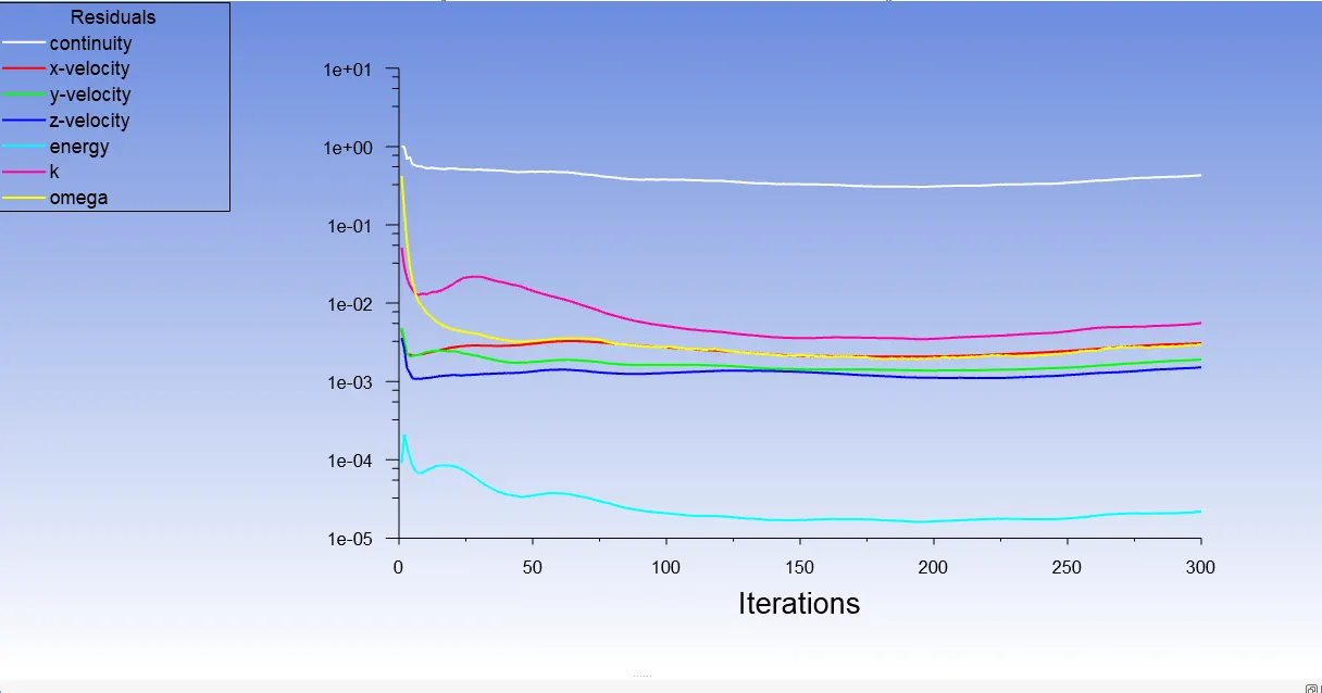
• For each simulation, you need to show the convergence plot.

Problem Setup

Understand k-epsilon and k-omega SST by considering case-1

1. Case 1 
   • Short mixing tee with a hot inlet velocity of 3m/s.
   • Momentum ratio of 2, 4. 
2. Case 2 
   • Long mixing tee with a hot inlet velocity of 3m/s.
   • Momentum ratio of 2, 4.

For momentum ratio 2

since, Mometnum ratio = Velocity of cold inlet / Velocity of hot inlet

2= Velocity of cold inlet/3

Velocity of cold inlet = 6 m/s

For momentum ratio 4

4= Velocity of cold inlet/3

Velocity of cold inlet = 12 m/s

Step1: Pre-processing

• First we took the geometry and we have to clean the body that means we need to convert mechanical body to desirable cad model.
• For this we use spacecliam to make cad model.

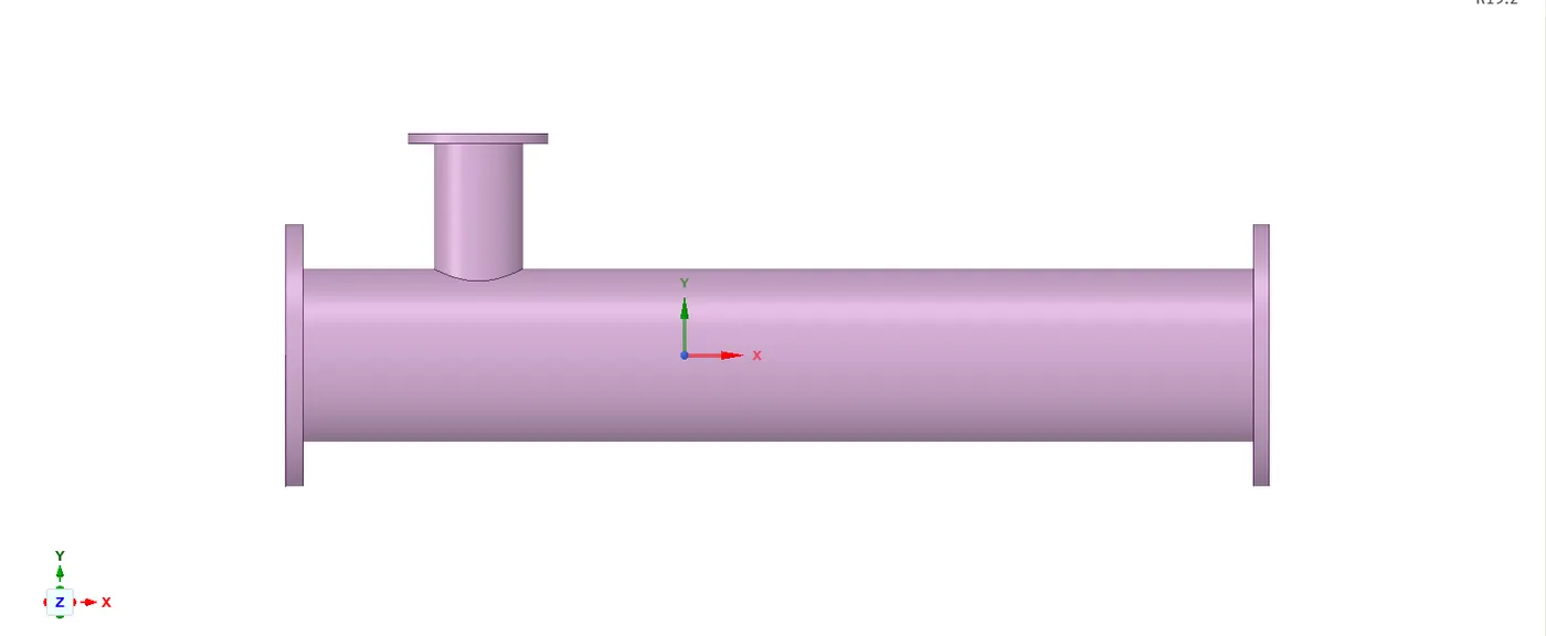
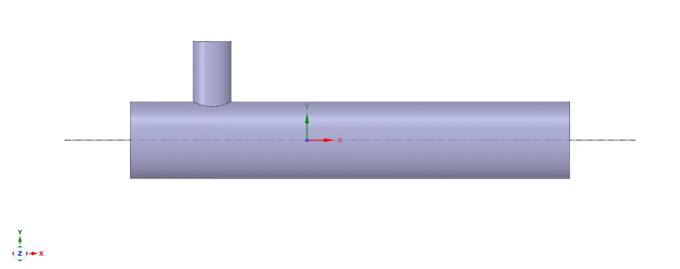
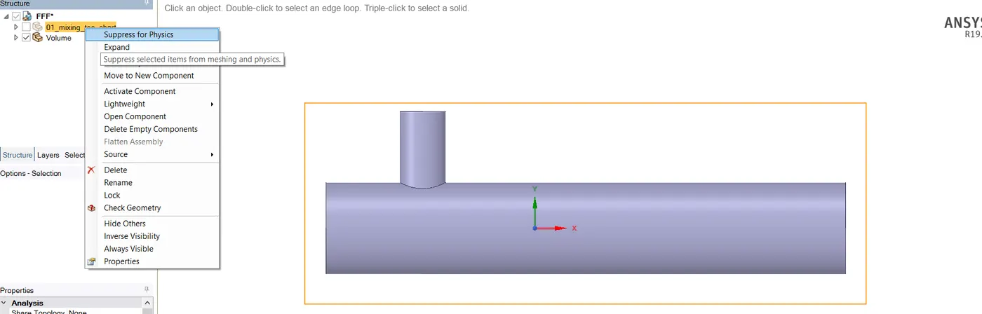
Suppress the actual model, as we do not have to make any conduction simulation in this project. Lastly, close the space Claim.

Mesh

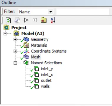
Create mesh, by using the sizing option we can adjust the element size. Also, create names such as inlet_y inlet_x, walls and outlet.

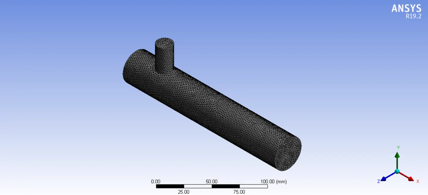
• To get the converged results we need good quality of mesh with good quality of mesh elements.
• Here in below we can see the quality of mesh elements in mesh matric.

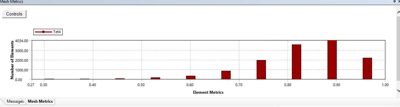
• Here more number of elements quality is good and all elements quality is above 30%. So we can use this mesh for further study.

Step2:  Solving

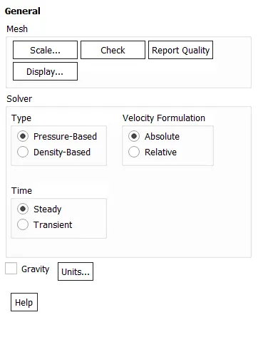
• In Setup, in physics select the energy model, as we have the heat transfer.
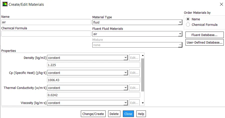
• Give the material, for the current model let the fluid be air.
• Under the viscous model, turbulent models have many different models, for the current model we select the K-epsilon à standard model.

Where K- turbulent kinetic energy

Epsilon – the rate of dissipation of kinetic energy.

• K epsilon model is better when the region of interest flow is away from the wall boundaries and K-omega is better when the region of interest is close to the wall boundaries.
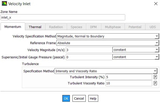
• Now go to boundaries option to set boundary conditions. Select inlet_x and click on option edit. It will open a menu, where all the parameter can be set whether it is thermal, radiation, momentum etc. Put the value of velocity as 3m/s and go to thermal parameter to set temperature as 36C, for hot fluid. For inlet_y set velocity as 6m/s as we are using momentum ratio of 2 and temperature as 19^oC.
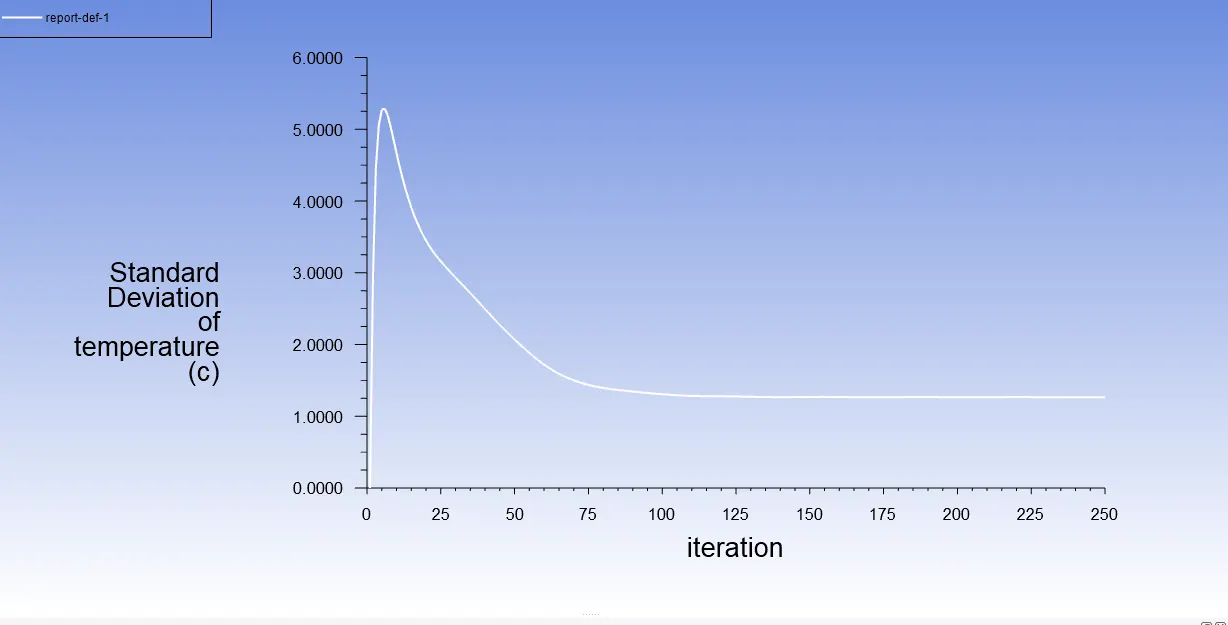
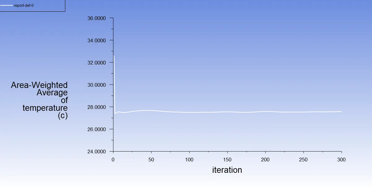
• Generating the temperature report of outlet and standard deviation of temperature. In solutions tab select definition and select area weighted average. In the opened menu select temperature as field variable. Similarly select standard deviation in definitions menu.
• Now click on initialization to calculate approximate values of velocity and pressure.
• Change the number of iterations to 250 and click on calculate. If solution is not converged, then iterations can be increased.
• Exit setup and double click on result to open CFD post. Check boxes to see walls and other parts. Click on walls and go to render set transparency of wall. Colour can also be changed to white for clear visibility.

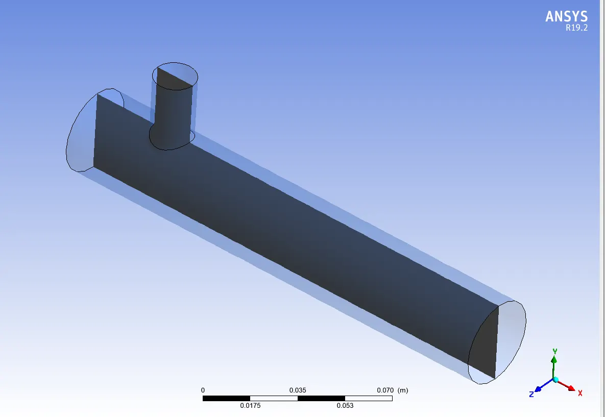
• Now insert a XY plane in wall by clicking on plane in location option of insert.
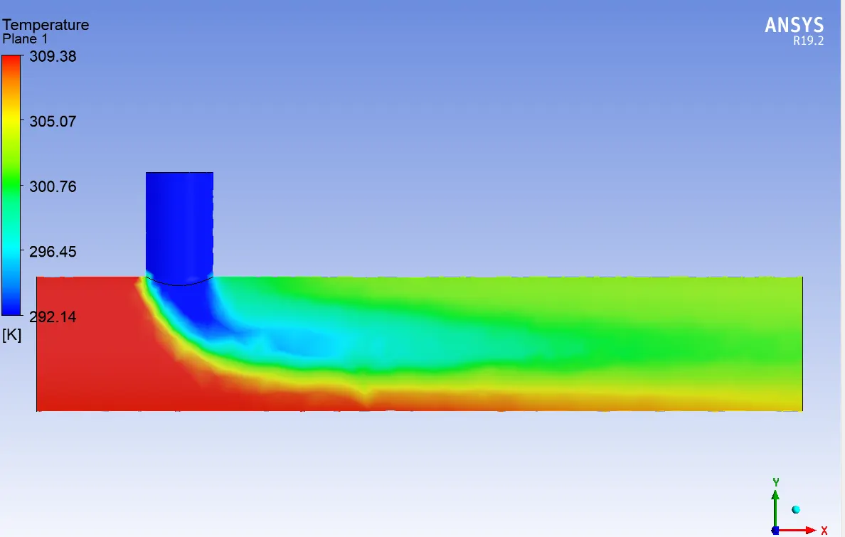
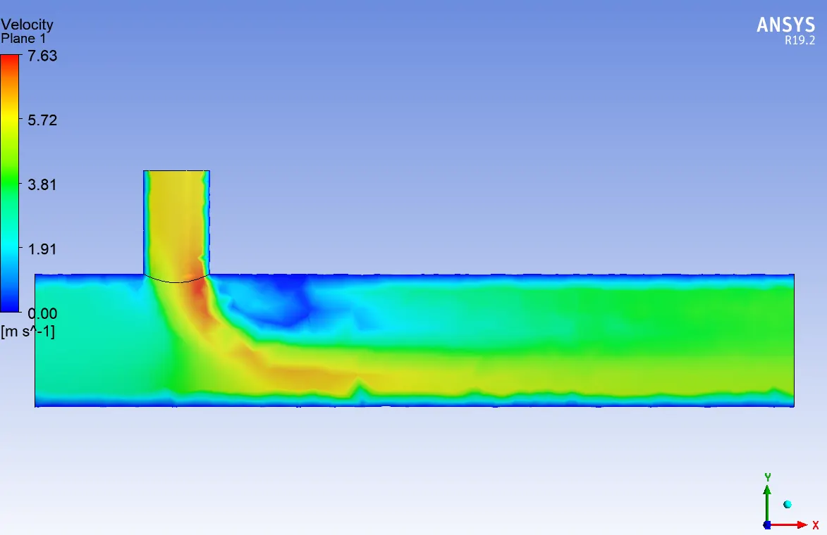
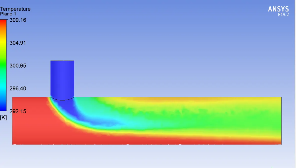
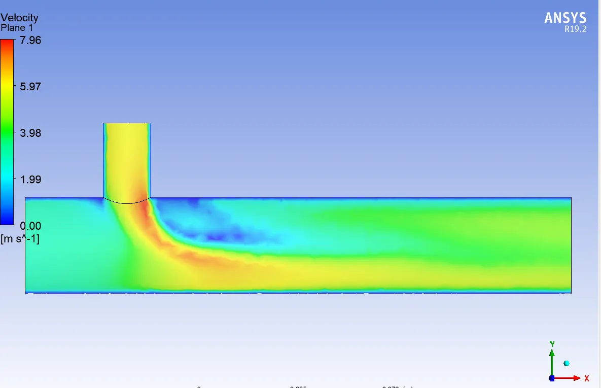
• Go to colour of plane and change it by variable choose option temperature. Similarly, velocity contours can be created by just changing variable as velocity.
• Right click on plane which we created and select streamline. Go to appearance and select temperature to see plot line on plane. Similar procedure can be repeated for velocity plot line.

RESULTS:

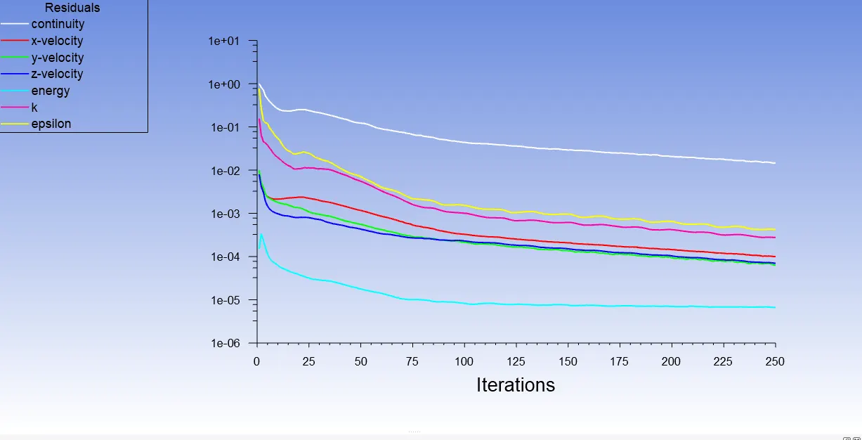
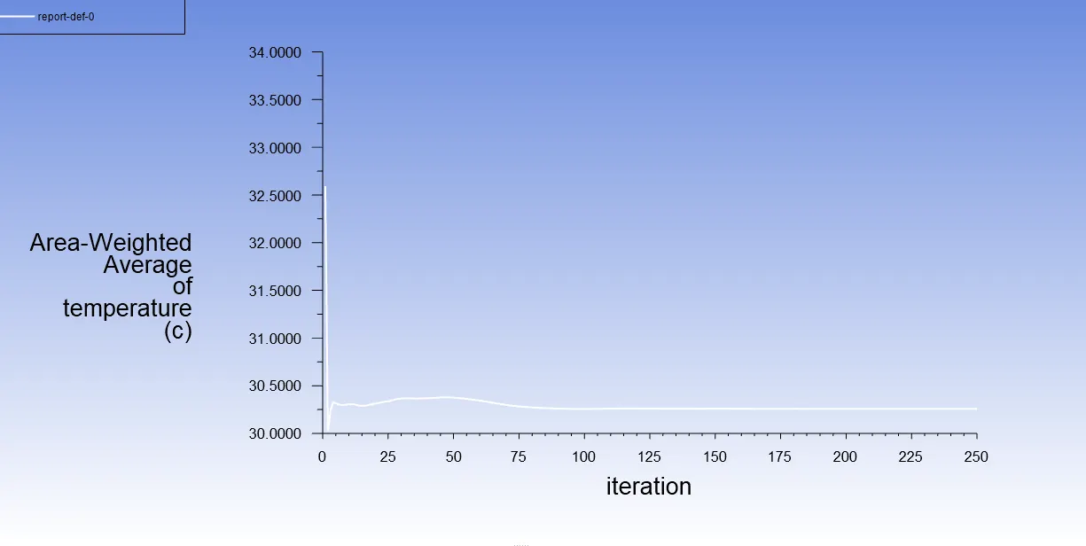
CASE1: In this short mixing tee is used, which was mixing two fluid with temperature 36C and 19C. Velocity of hot fluid was 3m/s and cold fluid was 6m/s. we used two different turbulent solvers for it first was realized k-epsilon and second was k-omega SST. The k-epsilon is giving better results because solution was converged after few iterations

Plot and contours from k-epsilon model:

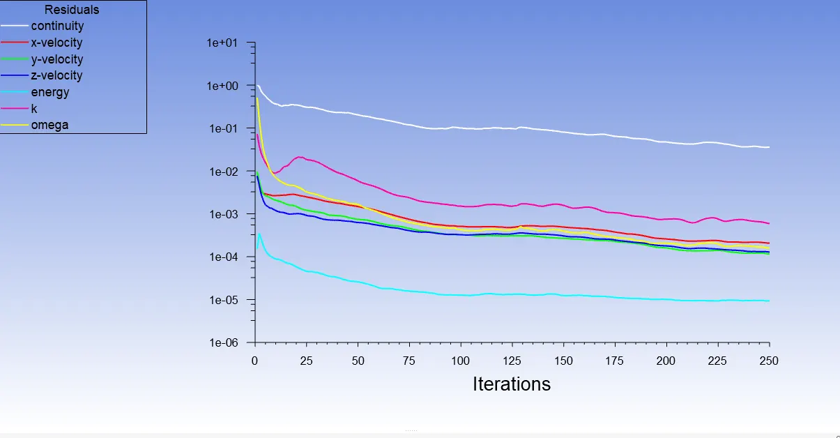
Residuals:

Average Temperature vs Iterations:

Standard Deviation of Temperature vs Iteration:

Temperature counter:

Velocity Counter:

Plot and contours from k-Omega SST model:

Using same above settings for K-Omega SST Method & comparing the results 

Residuals:

Average Temperature vs Iterations:

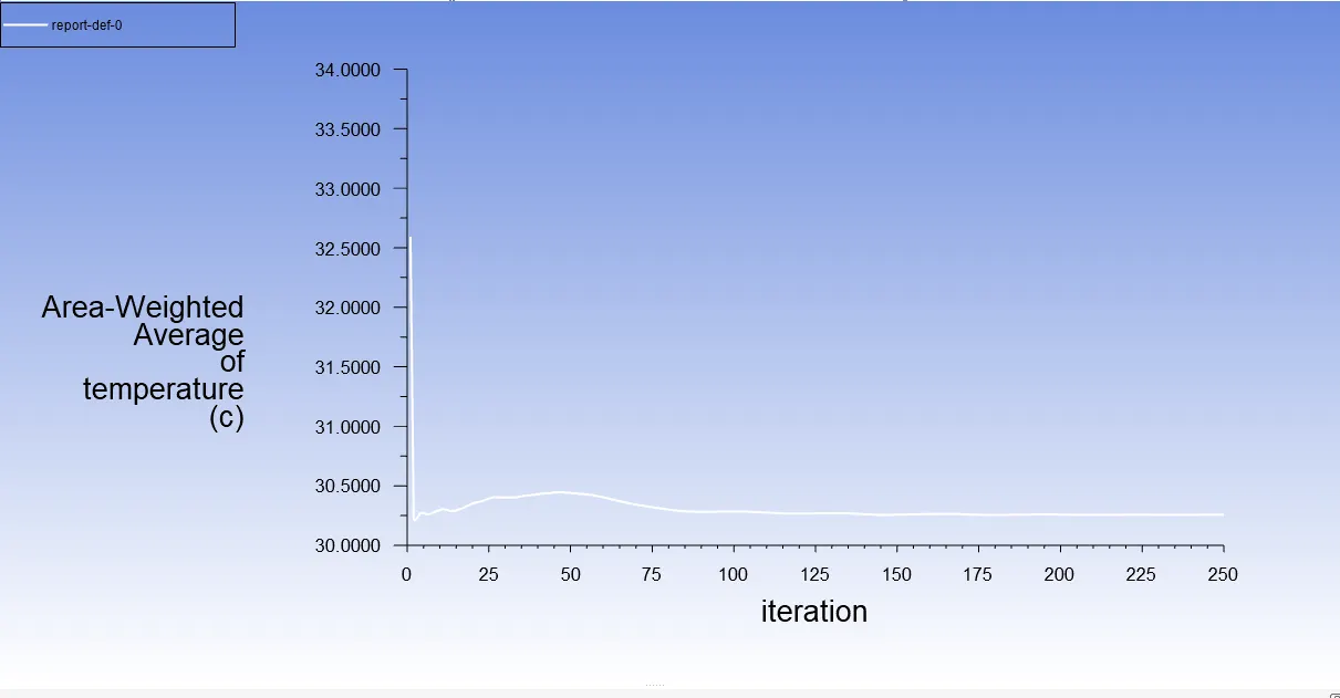
Standard Deviation of Temperature vs Iteration:

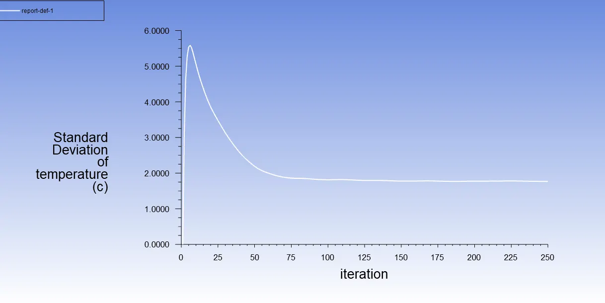
Temperature Counter :

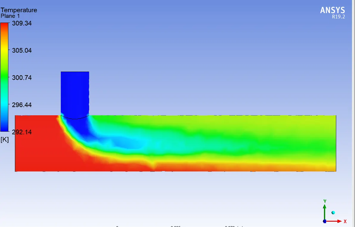
Velocity Counter :

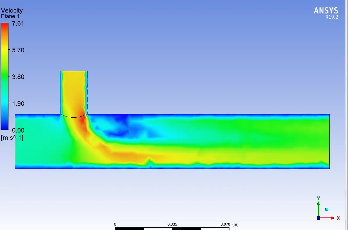
Case-1-a

Short mixing tee

a - Simulation-1

Inlet velocity - 3m/s

Momentum ratio - 2

Inlet velocity of cold air = 3x2 = 6 m/s

Results

Residue plot:

Average Temperature vs Iterations:

Standard Deviation of Temperature vs Iteration:

Temperature Counter :

Velocity Counter :

 

 Case-1-b

Short mixing tee

a - Simulation-1

Inlet velocity - 3m/s

Momentum ratio - 4

Inlet velocity of cold air = 3x4 = 12m/s

Results

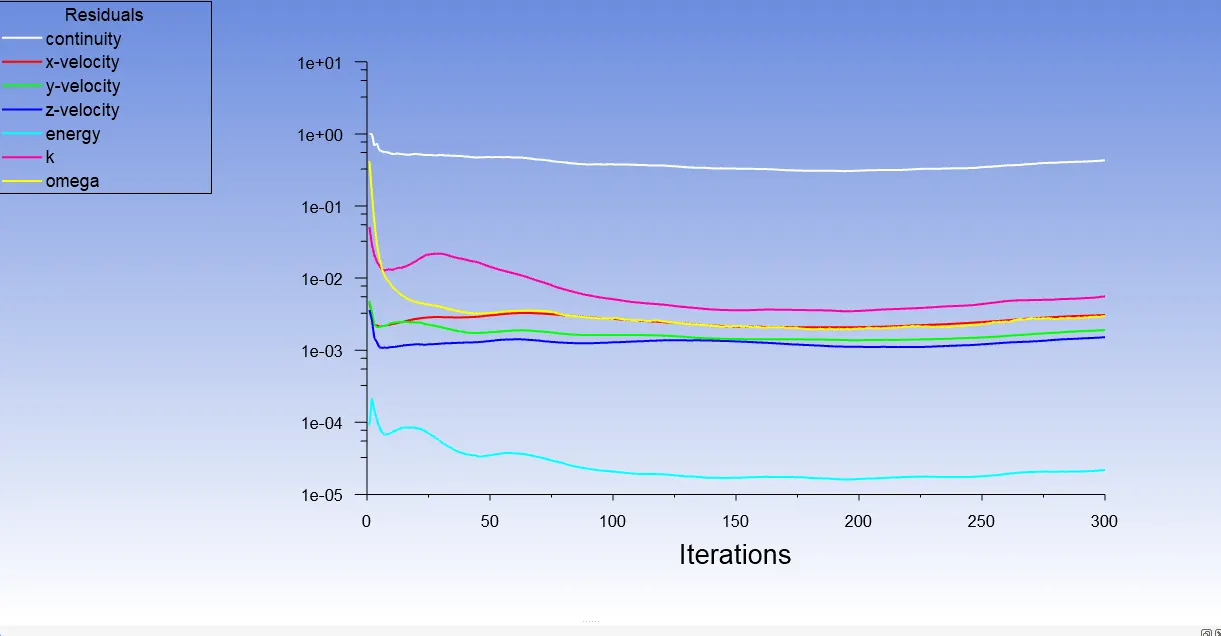
Residue plot:

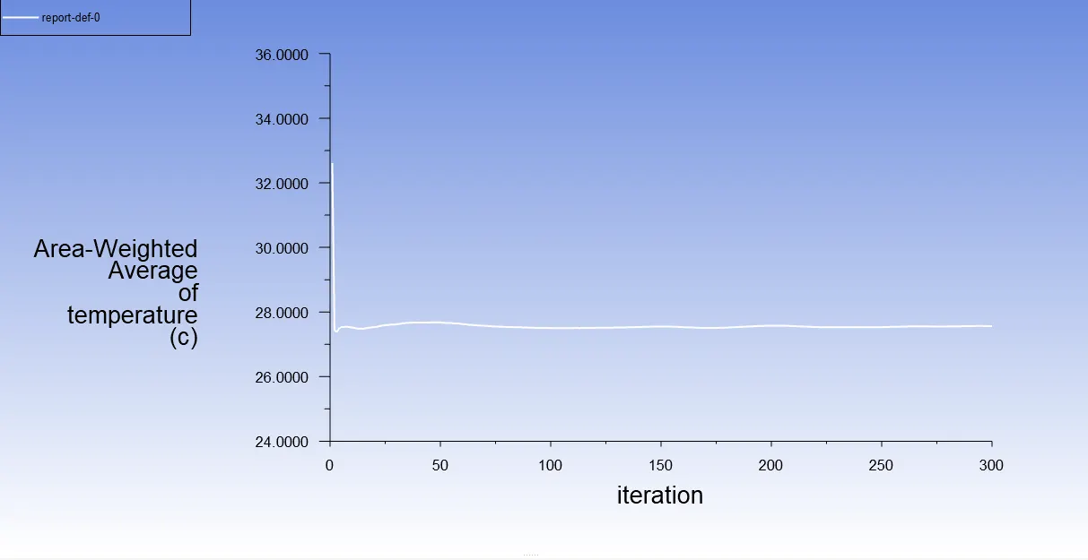
 Average Temperature vs Iterations:

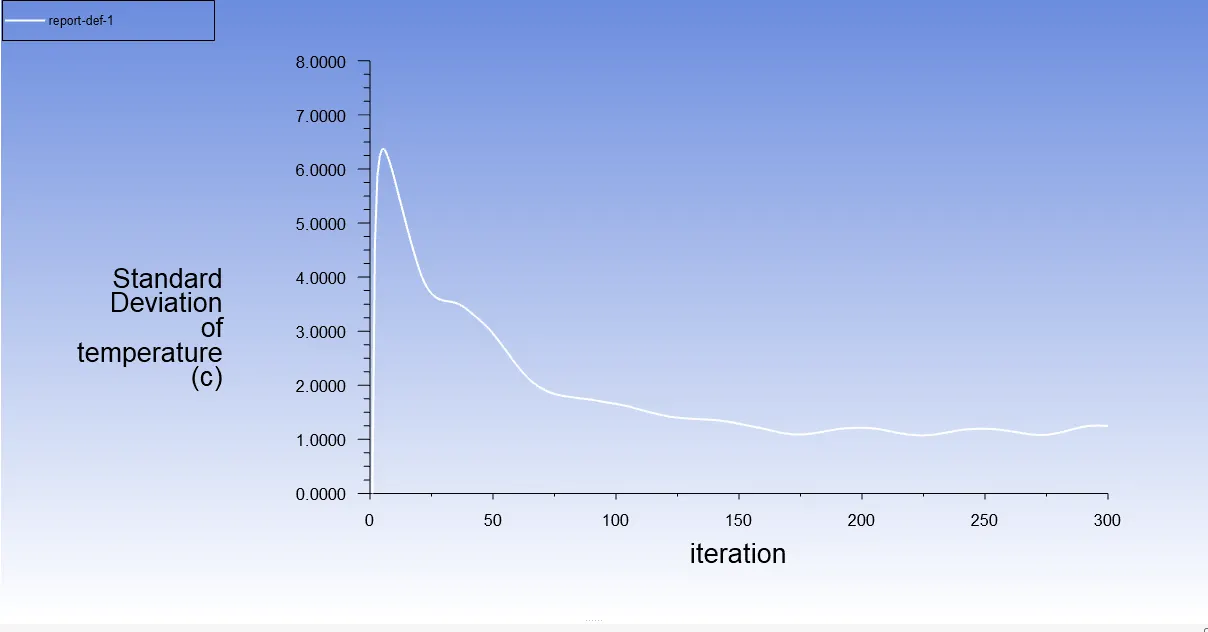
 Standard Deviation of Temperature vs Iteration:

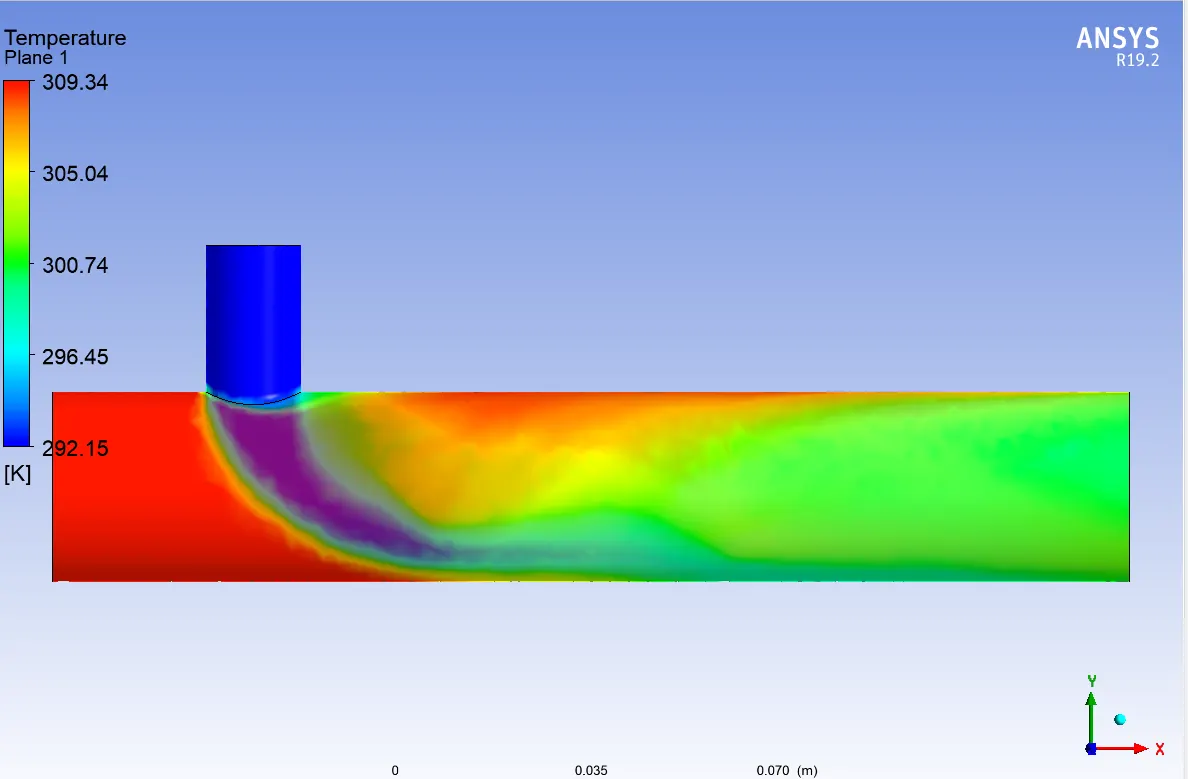
Temperature Counter :

 

Velocity Counter :

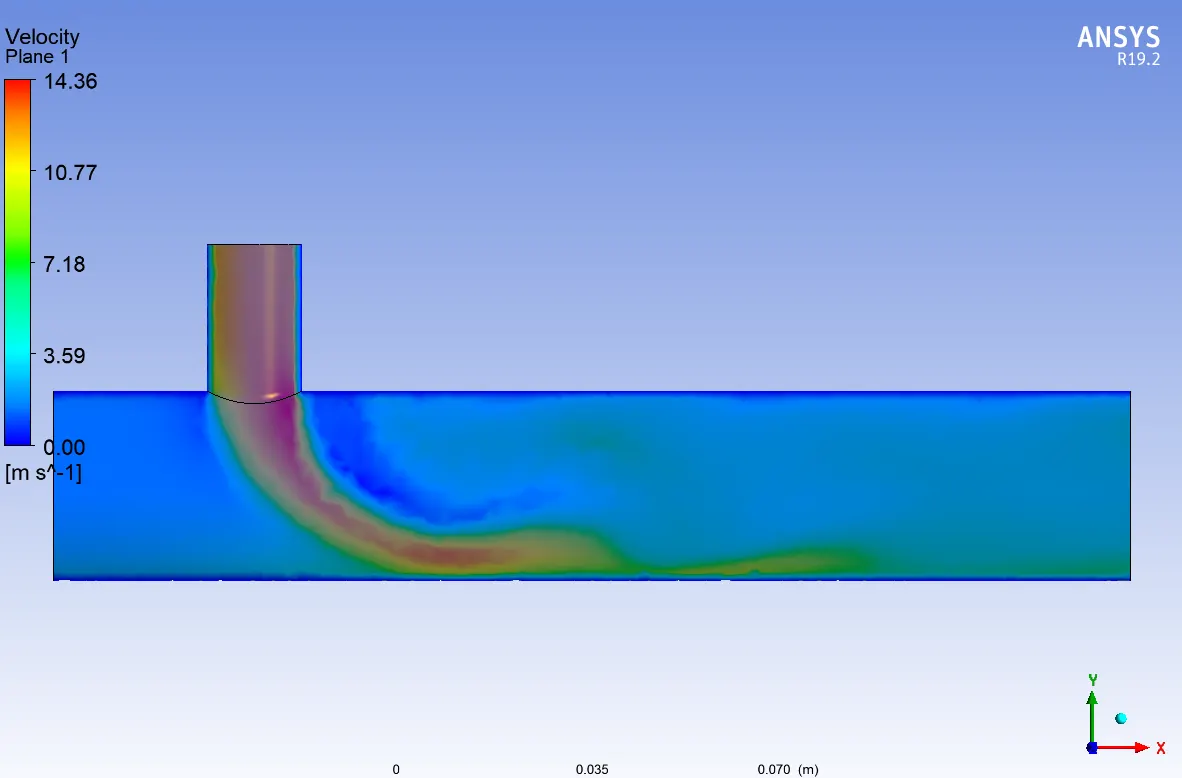
Case-2-a

Long mixing tee

a - Simulation-1

Hot Inlet velocity - 3m/s

Momentum ratio - 2

Inlet velocity of cold air = 3x2 = 6m/s

Results

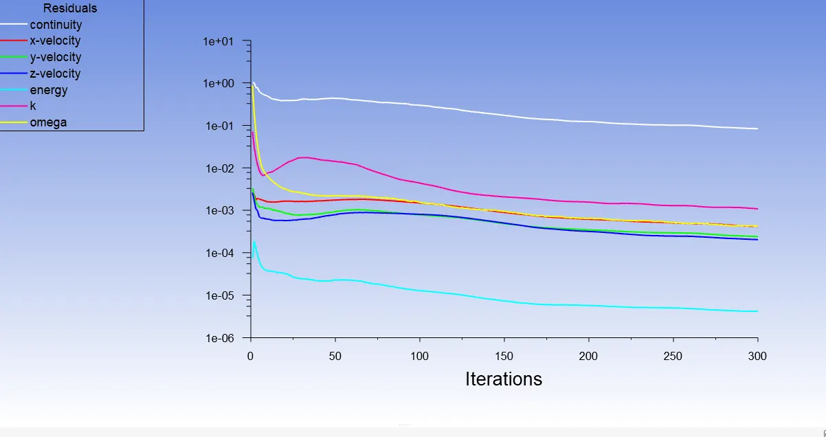
Residue plot:

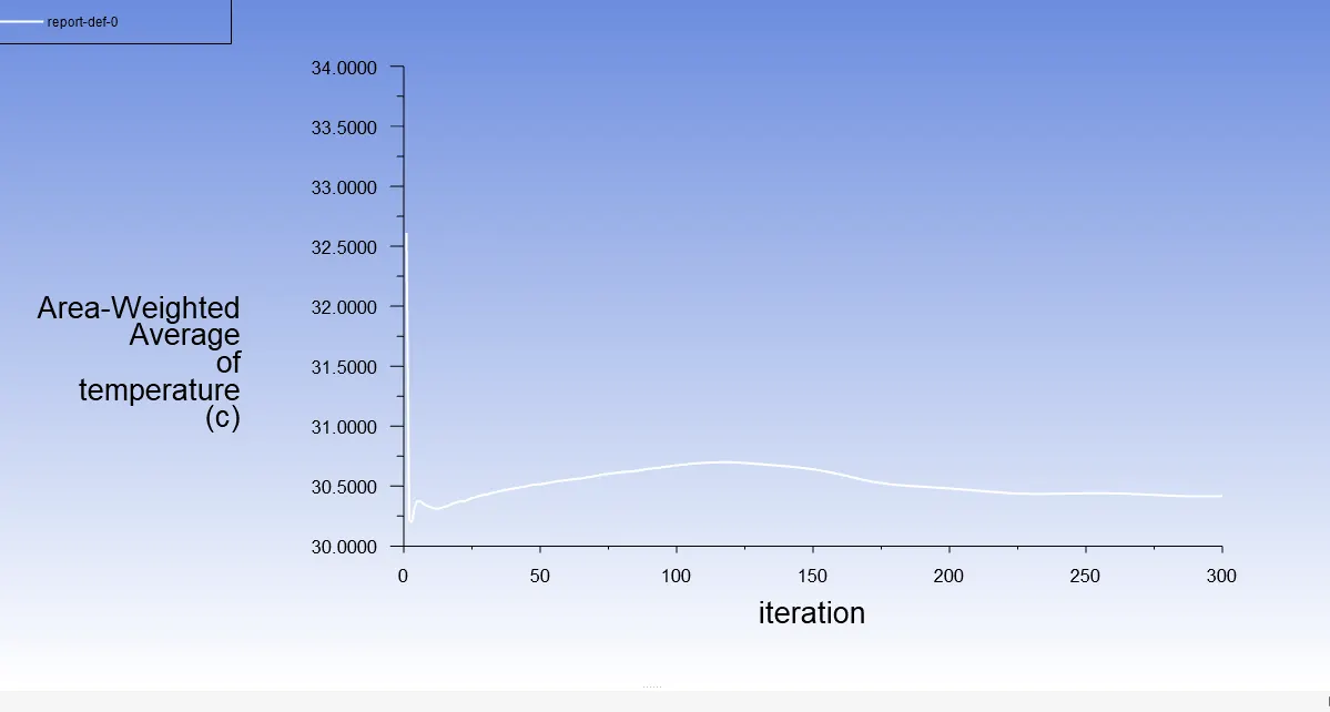
Average Temperature vs Iterations:

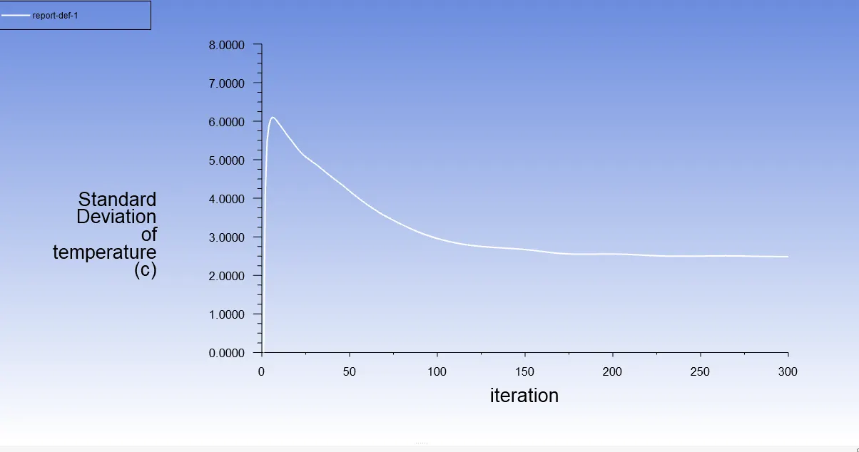
Standard Deviation of Temperature vs Iteration:

Temperature Counter :

Velocity Counter :

Case-2-b

Long mixing tee

a - Simulation-1

Hot Inlet velocity - 3m/s

Momentum ratio - 4

Inlet velocity of cold air = 3x4 = 12m/s

Results

Residue plot:

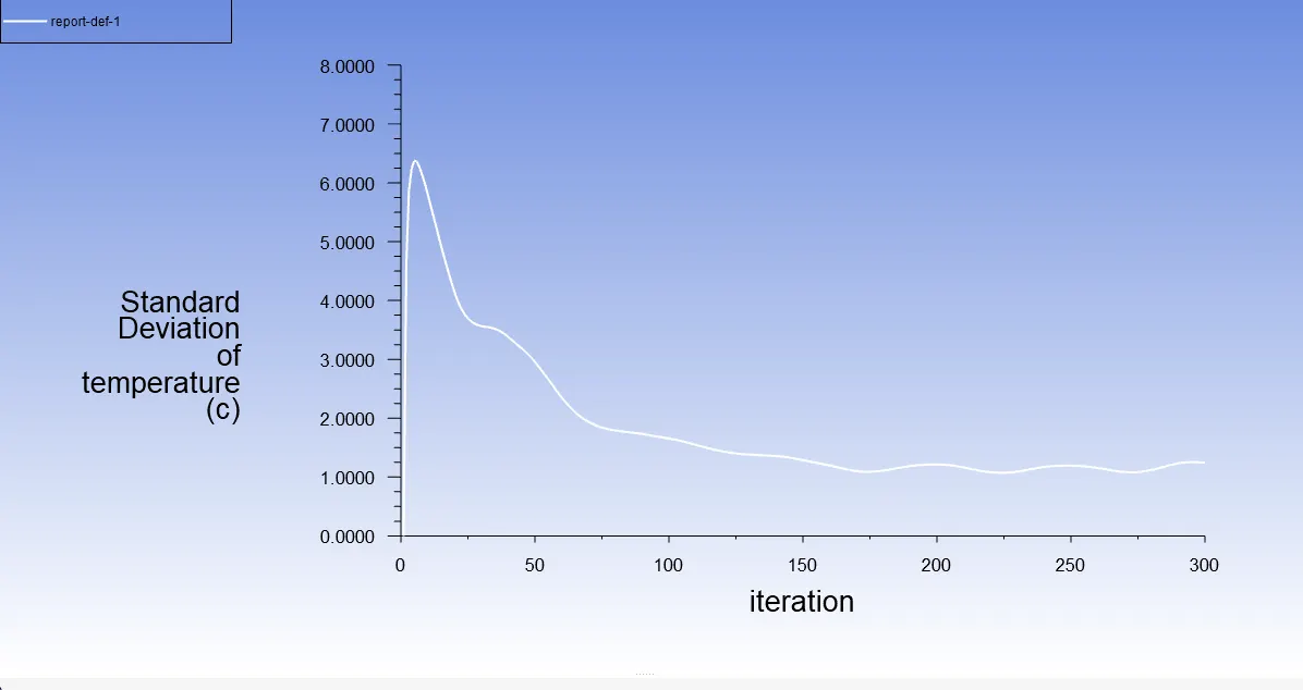
Average Temperature vs Iterations:

Standard Deviation of Temperature vs Iteration:

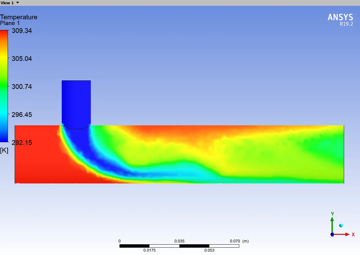
Temperature Counter :

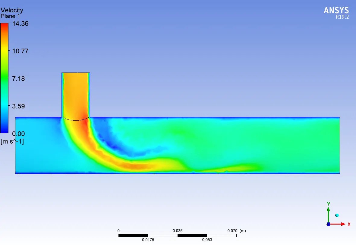
Velocity Counter :

Conclusion :

• k-epsilon models predict flow virtually far from the boundaries (wall), and the k-omega model predicts near the wall. As in this case we need a flow simulation turbulent model far from the wall, therefore, the k-epsilon method is used.

• As seen in the Case-1-a and Case-1-b, the temperature at the outlet drops down significantly due to high velocity of cold air from the inlet. This is possible due to the turbulent mixing at the tee joint between hot air and cold air because of the high velocity of cold air., which is not possible in case of low-velocity cold air.