Week 1- Mixing Tee

Aim:  to set up steady-state simulations to compare the mixing effectiveness.

Objective: Given that there are two version of  mixing tee, one is comparatively longer than other.

• To perform fluid flow simulation with the k-epsilon and k-omega SST model.
• To perform fluid flow simulation for both the cases
• Case 1: 
  • Short mixing tee with a hot inlet velocity of 3m/s.
  • Momentum ratio of 2, 4. 
• Case 2: 
  • Long mixing tee with a hot inlet velocity of 3m/s.
  • Momentum ratio of 2, 4.

•  To compare the following values from the 2 cases. 

  1. Cell count
  2. Average outlet temperature
  3. Number of iterations for convergence

Given: 

• Hot inlet temperature : 36°C 
• Cold inlet temperature : 19°C

Formula: 

• Momentum ratio = velocity at cold inlet / velocity at hot inlet.

Turbulence Models used for simulation and reason:

1. K-epsilon model (K-ε) : It is most commonly used turbulence model in computational fluid dynamics (CFD) to simulate mean flow characteristics for turbulent flow conditions. it is a two equation model that gives a general description of turbulence by means of two transport equations. it exibits superior performance for flows involving rotation, boundary layers under strong adverse pressure gradients, seperation and recirculation. In every measure of comparison, Realizable K-ε demonstrates a superior ability to capture the mean flow of the complex structures.  
2. K-omega model : It is one of the most commonly used models to capture the effects of turbulent flow conditions. it is two equation model. it is more efficient in predicting stronger seperation. also performs well for swirling flows and in the near wall region.
3. Spalart-Allmaras model : It is the commonly used turbulence model in aerodynamics. it is choosen because it is used in boundary layer flows with arbitrary pressure gradient. it gives clearance of flows and also avoids leakages in flows which helps in obtaining proper results.

Case 1.1:

• Short mixing tee
• Hot inlet velocity = 3 m/s
• Momentum ratio = 2
• Cold inlet velocity = 2 × 3 = 6 m/s 
• Hot inlet temperature : 36°C 
• Cold inlet temperature : 19°C
• Turbulence model: k-epsilon

Case 1.2:

• Short mixing tee
• Hot inlet velocity = 3 m/s
• Momentum ratio = 4
• Cold inlet velocity = 4 × 3 = 12 m/s 
• Hot inlet temperature : 36°C 
• Cold inlet temperature : 19°C
• Turbulence model: k-epsilon

 Case 2.1:

• long mixing tee
• Hot inlet velocity = 3 m/s
• Momentum ratio = 2
• Cold inlet velocity = 2 × 3 = 6 m/s 
• Hot inlet temperature : 36°C 
• Cold inlet temperature : 19°C
• Turbulence model: k-epsilon

Case 2.2:

• long mixing tee
• Hot inlet velocity = 3 m/s
• Momentum ratio = 4
• Cold inlet velocity = 4 × 3 = 12 m/s 
• Hot inlet temperature : 36°C 
• Cold inlet temperature : 19°C
• Turbulence model: k-epsilon

Case 3:

• Short mixing tee
• Hot inlet velocity = 3 m/s
• Momentum ratio = 2
• Cold inlet velocity = 2 × 3 = 6 m/s 
• Hot inlet temperature : 36°C 
• Cold inlet temperature : 19°C
• Turbulence model: spalart-allmaras

Procedure:

1. Procedure for case 1.1:

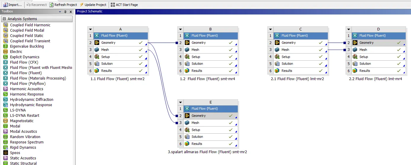
• Open ansys workbench and drag and drop the fluid flow fluent menu.
• 

Spaceclaim:

• open spaceclaim to edit the autocad model and to make it suitable for simulation.
• here we have to perform inner flow simulation so that we do not need the thickness of model.
• hence to remove thickness, select prepare deck then select éxtract volume' option and do the selection using edge selection of required model.
• then hide the solid part and supress it for physics so that it will not interfair in simulation.
• 
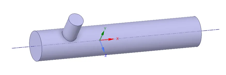
• then close the spaceclaim and the geometry will directly get upload for meshing.

Mesh:

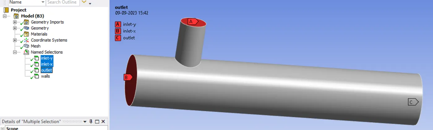
• open mesh and then first thing we need to do is assigning names i.e. named selection as shown below
• 
• then entered element size as 0.005 m and generated mesh using 'generate mesh' menu.
• 
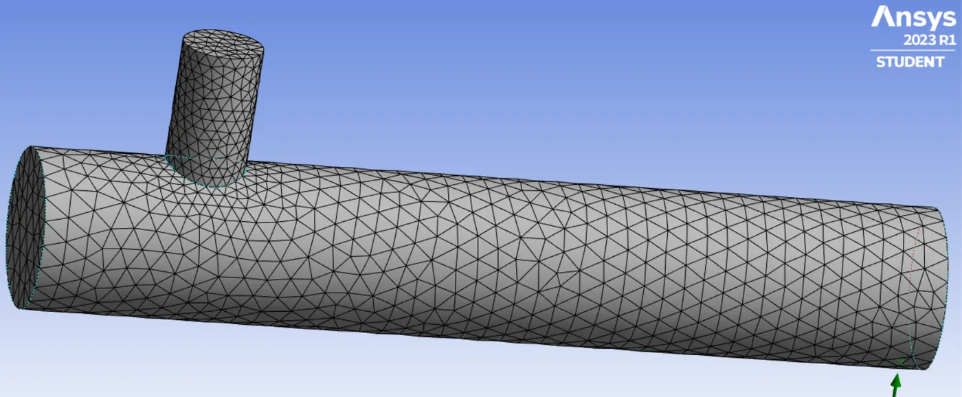
• then closed the mesh window and updated the mesh in workbench.

Setup:

• open setup with double precision and it will show everything about meshing like no. of cells, no. of nodes, etc
• then go to general > type - pressure basedd > velocity formulation - absolute > time - steady > tick energy equation.
• models > viscous model - k-epsilon > reliazable > standard wall function.
• Material > Air > material type -fluid > density - constant(1.225 kg/m⊃3;).
• Cellzone > volume_volume > type - fluid.
• Boundary conditions > inlet-x > type - velocity inlet > velocity specification - magnitude, normal to boundary > velocity magnitude - 6 m/s > temperature - 19°C. 
• Boundary conditions > inlet-y > type - velocity inlet > velocity specification - magnitude, normal to boundary > velocity magnitude - 3 m/s > temperature - 36°C. 
• Boundary condition > outlet > type - pressure outlet > gauge pressure - 0 pa.
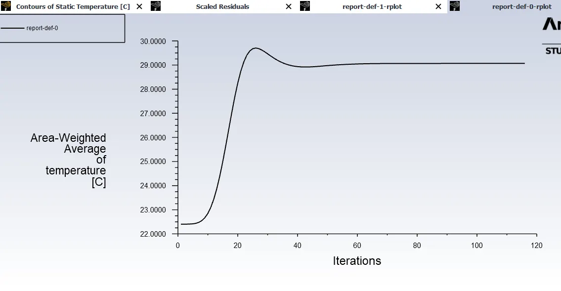
• Report defination 1: new > surface report > Area weighted average > field variable - Temperature > surface - outlet > create - report files and report plot.
• Report defination 2: new > surface report > standard deviation > field variable - Temperature > surface - outlet > create - report files and report plot.
• Initialization > hybrid initialization method > initialize.
• Run calculation > no. of iteration > 350 > run calculation. 
• Results > create > plane > xy-plane (to plot contour along the length of pipe) 
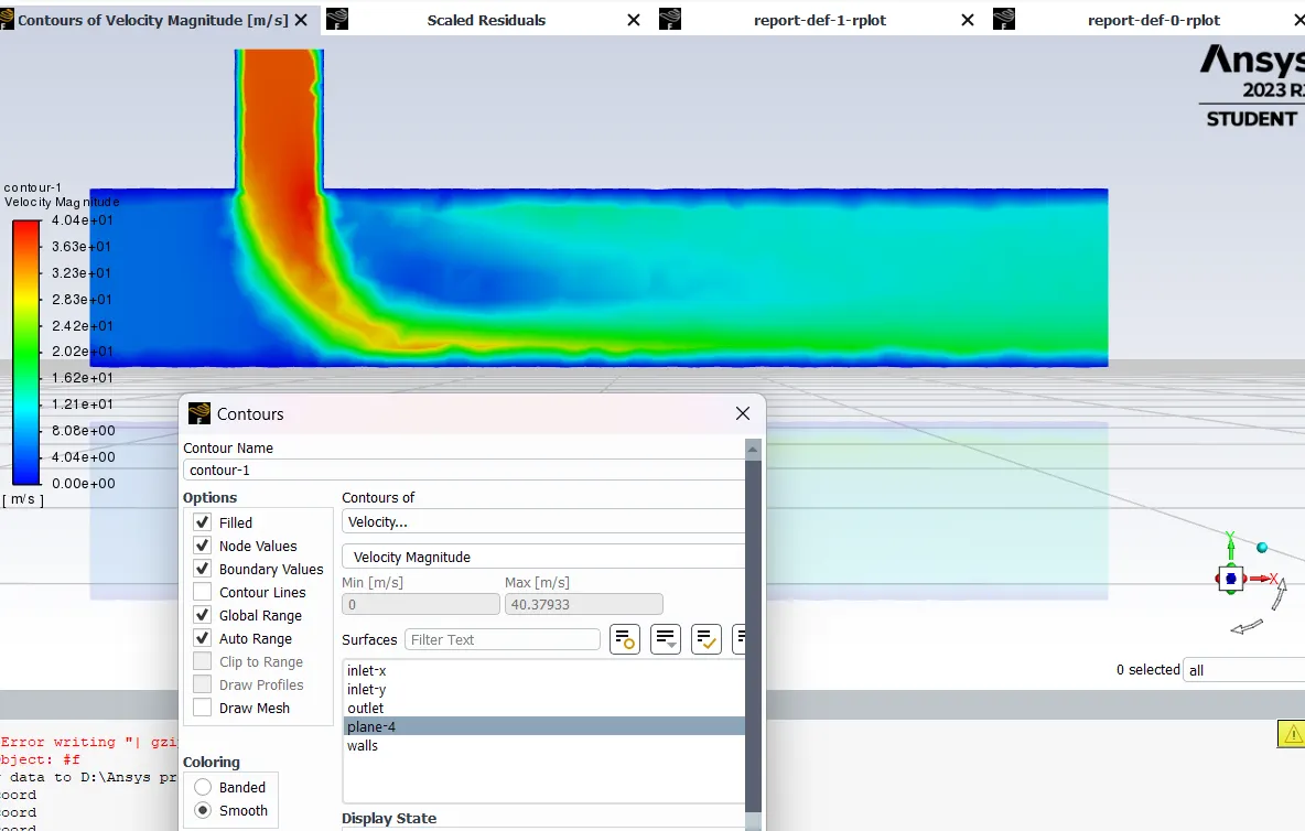
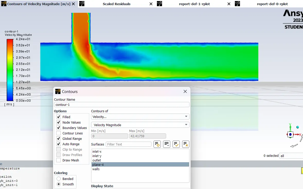
• Results > contour > new > contour of - velocity > surface - plane 4 (xy plane) > save and display.
• 
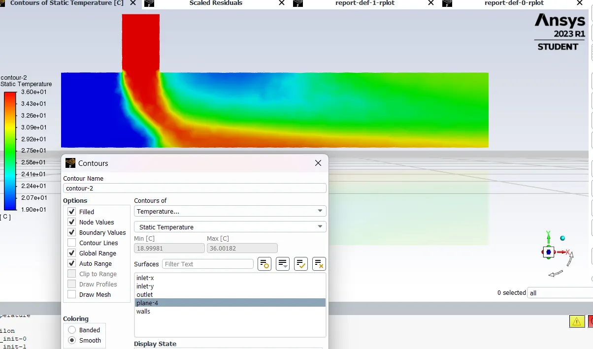
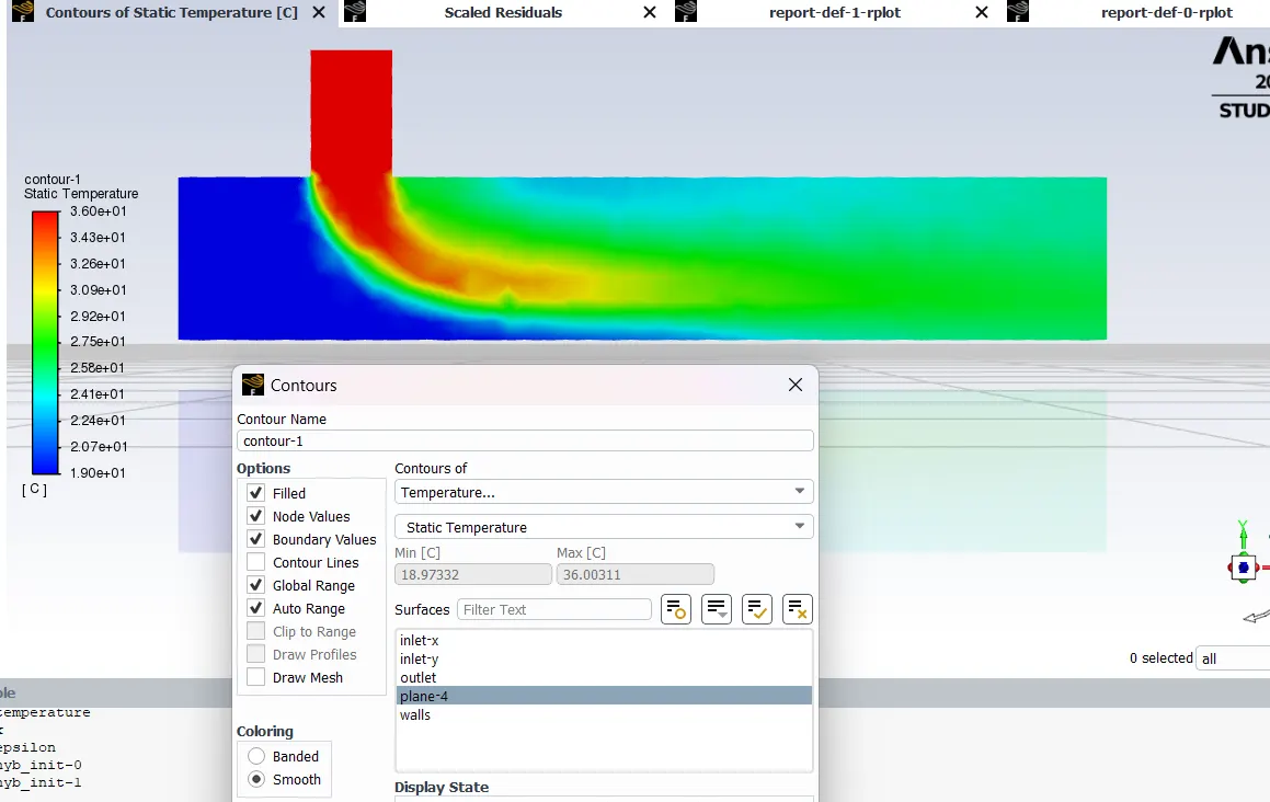
• Results > contour > new > contour of - temperature > surface - plane 4 (xy plane) > save and display.
• 
• Results > create > plane > yz-plane (to plot contour across the length of pipe) 
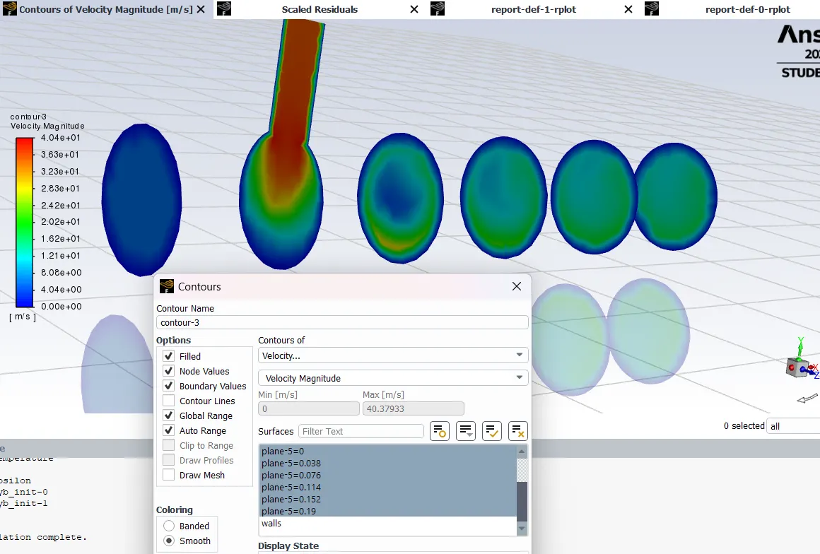
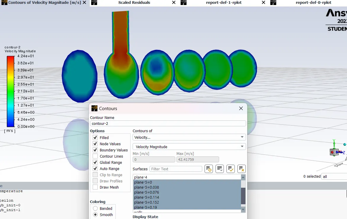
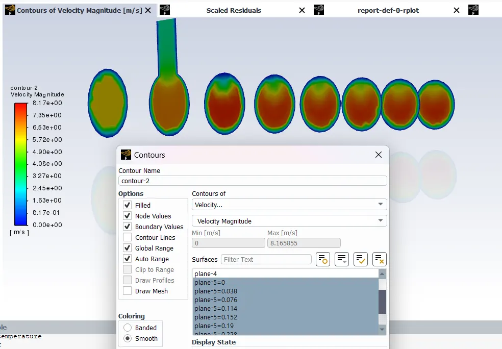
• Results > contour > new > contour of - velocity > surface - plane 5 (all yz planes of plane 5) > save and display.
• 
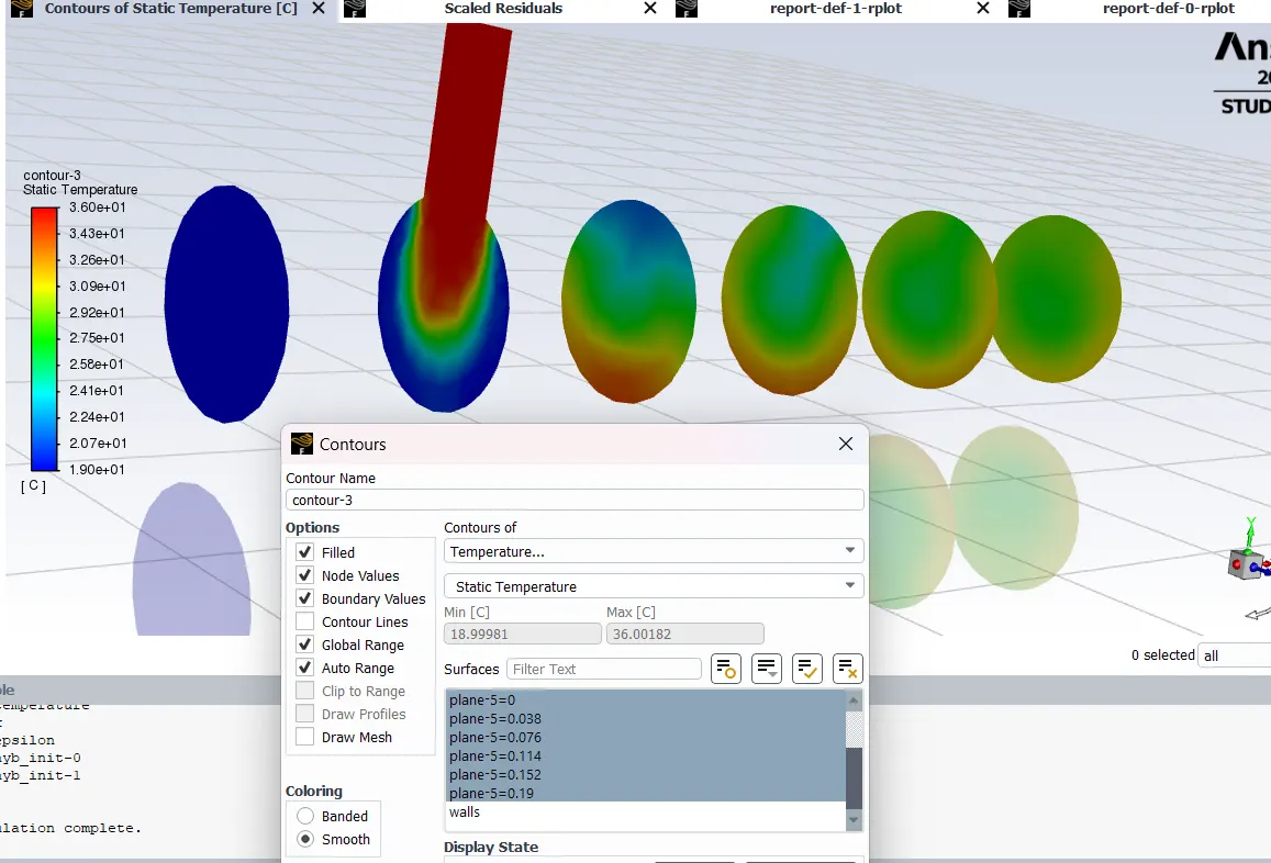
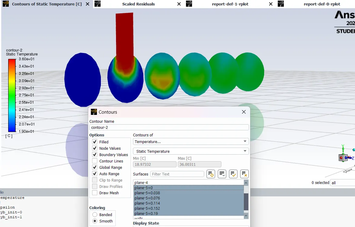
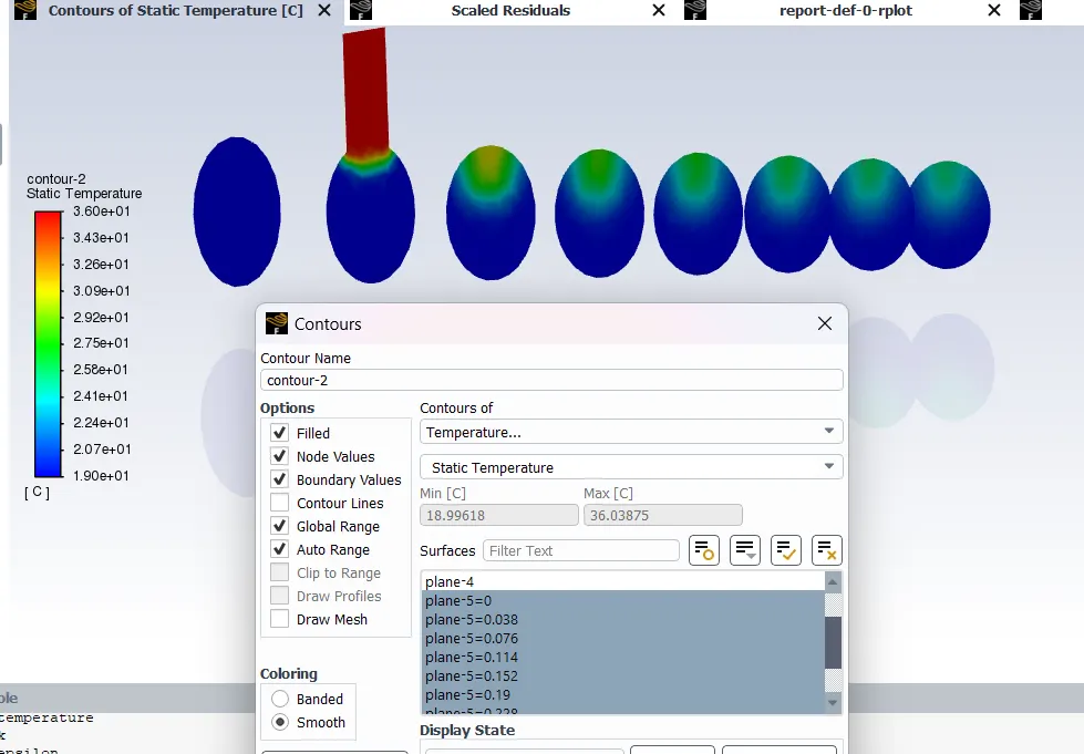
• Results > contour > new > contour of - temperature > surface - plane 5 (all yz planes of plane 5) > save and display.
• 
• Temperature line plot:
• 
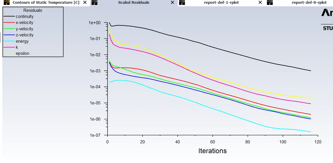
• convergence :
• 

 2. Procedure for case 1.2:

• Geometry, mesh and setup is copied from the fluent menu from case 1.1 using duplicate option.
• In this case , as the momentum ratio changes so the cold inlet velocity will change.
• so we just need to change the velocity for inlet-x in  the boundary conditions.
• then do the initialization at t=0 and run the calculation for 350 iterations.
• Then repeated same process to get required plots and contours.
• velocity contour along the length of pipe
• 
• temperature contour along the length of pipe
• 
• velocity contour across the length of pipe
• 
• temperature contour across the length of pipe
• 
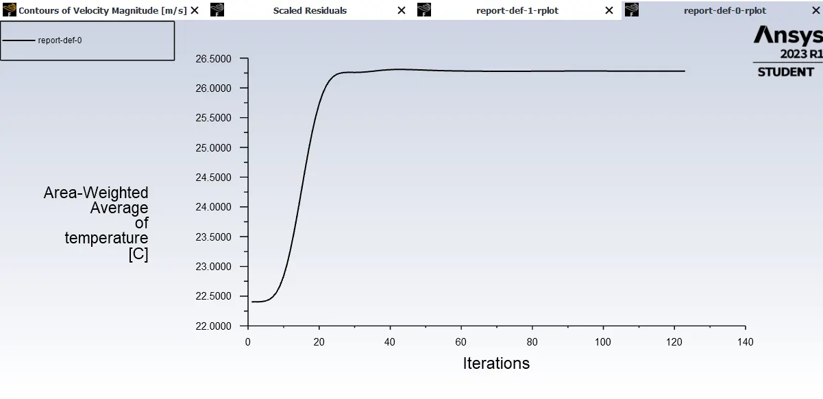
• Temperature line plot:
• 
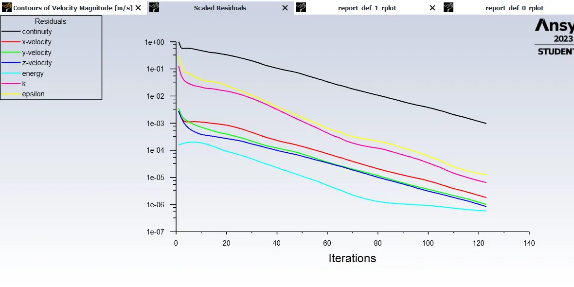
• Convergence plot:
• 

3. Procedure for case 2.1:

• Open another fluid flow fluent menu on the same workbench.
• repeated the same procedure as for case 1.1 just replacing short mixing tee with long mixing tee.
• updated spaceclaim model:
• 
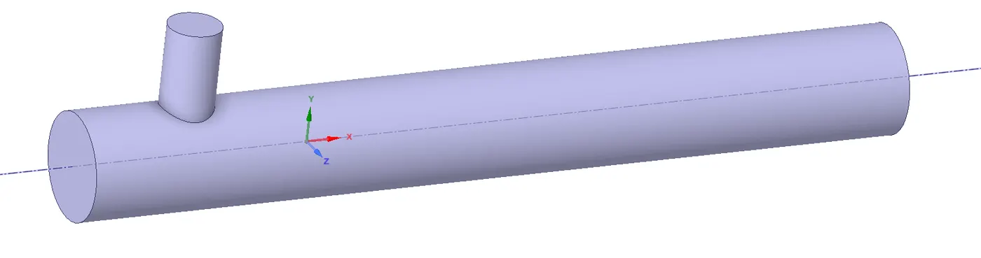
• proceed with the named selsction and meshing.
• 
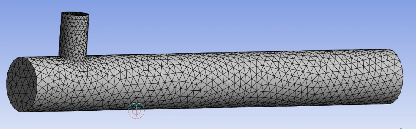
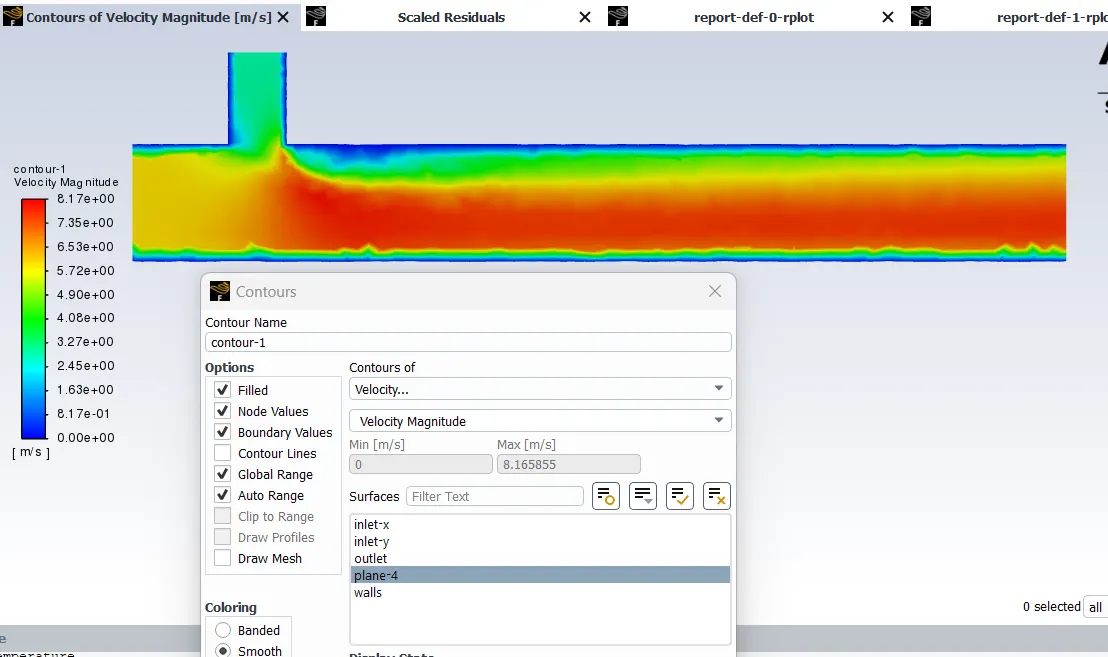
• Repeated the same process as for case 1.1 with the same input and get required plots and contours.
• Velocity contour along the length of pipe:
• 
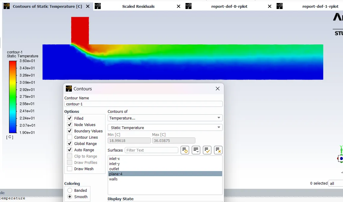
• Temperature contour along the length of pipe:
• 
• Velocity contour across the length of pipe:
• 
• Temperature contour across the length of pipe:
• 
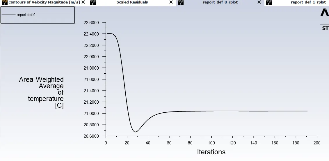
• Temperature line plot:
• 
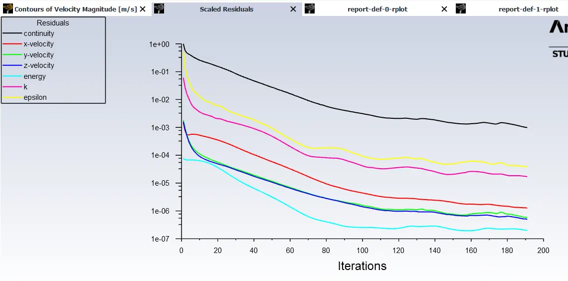
• Convergence plot:
• 

4. Procedure for case 2.2:

• Geometry, mesh and setup is copied from the fluent menu from case 2.1 using duplicate option.
• In this case , as the momentum ratio changes so the cold inlet velocity will change.
• so we just need to change the velocity for inlet-x in  the boundary conditions.
• then do the initialization at t=0 and run the calculation for 350 iterations.
• Then repeated same process to get required plots and contours.
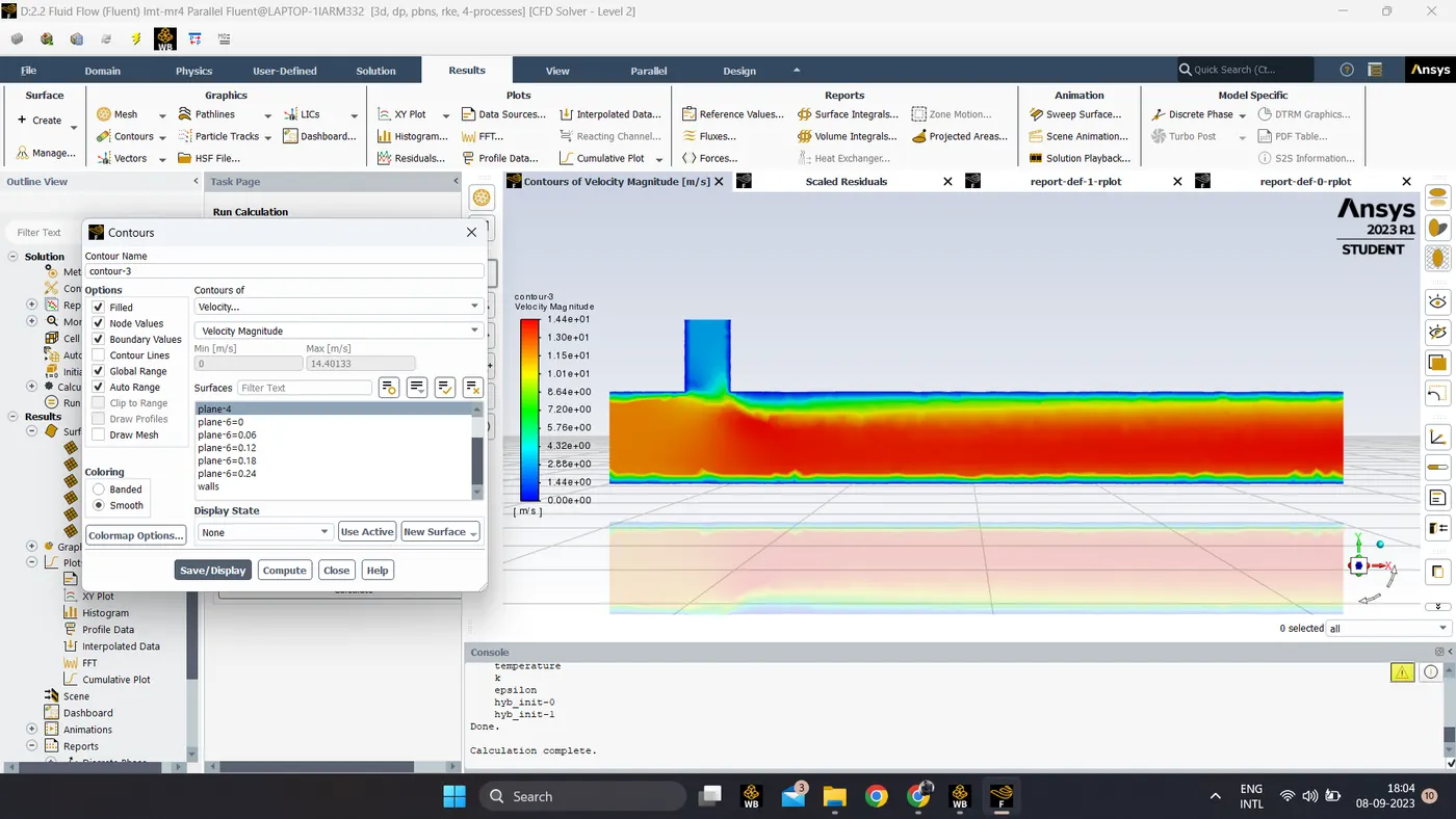
• Velocity contour along the length of pipe:
• 
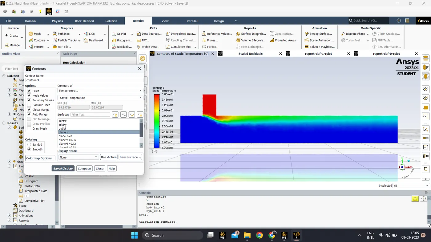
• Temperature contour along the length of pipe:
• 
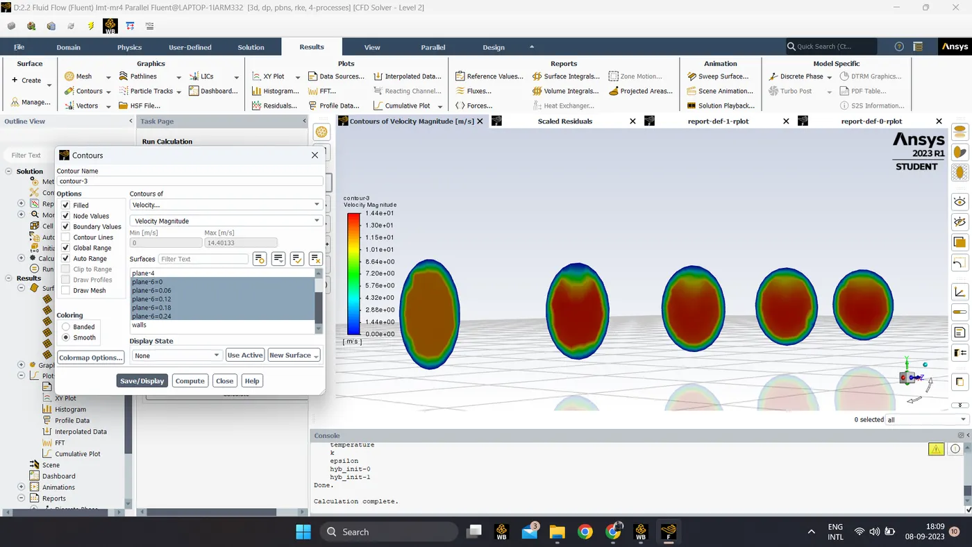
• Velocity contour across the length of pipe:
• 
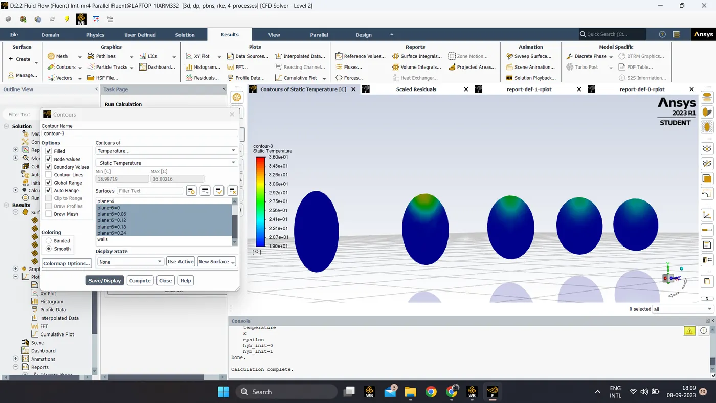
• Temperature contour across the length of pipe:
• 
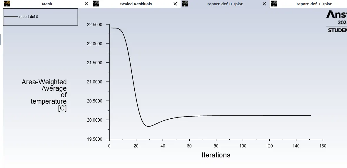
• Temperature line plot:
• 
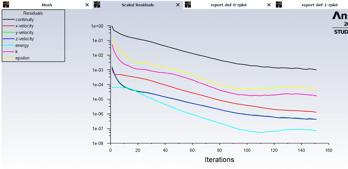
• Convergence plot:
• 

5. Procedure for case 3:

•  Case 3 is done with the same model and inputs as in case 1.1 but only change is turbulence model.
• So here spalart-allmaras turbulence model is used instead of k-epsilon to check the differences cause due to changing turbulence model.
• The number of cells and average output temperature was same but the number of iteration it took to get converge is bit more.
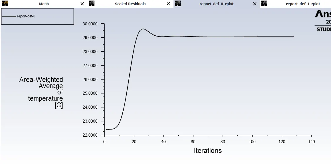
• Temperature line plot:
•  
• Convergence plot:
• 
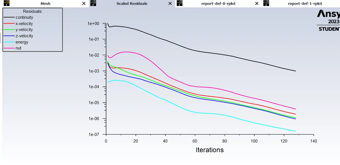
• So anyone can easily understand from covergence plot that it is getting converge in 128 iterations and from temperature plot that the average temperature is 29°C.

Table:

	Case 1.1	Case 1.2	Case 2.1	Case 2.2	Case 3
Cell count	14248	14248	17904	17904	14248
Aversge output temperature	29	26.25	21	20	29
No. of iteration for convergence	116	123	191	151	128

Conclusions:

• As the length of mixing tee increases, number of cell count increases with same element size.
• As the length of mixing tee increases, average output temperature decreases.
• With same length of mixing tee, if the velocity of cold fluid ( i.e. at inlet-x) increases, then the average output temperature comparatively decreases.
• number of iteration for convergence are increses with increase in length of mixing tee.

Mesh Independent Study:  

• It is a study to check whether the simulaion results are independent of the undelying mesh or not.
• we can perform mesh independent study by changing the element size of mesh (i.e. mesh resolution).
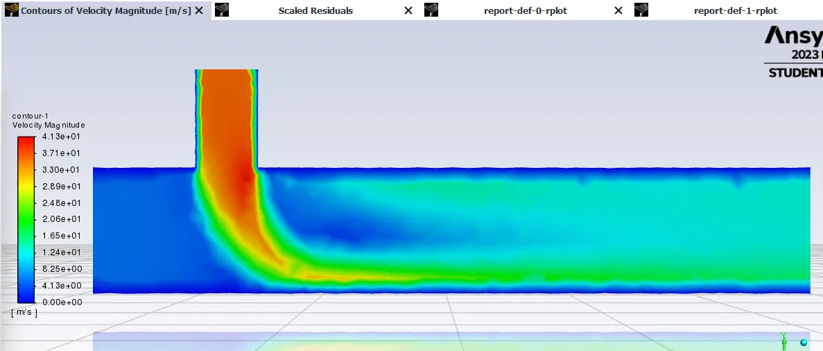
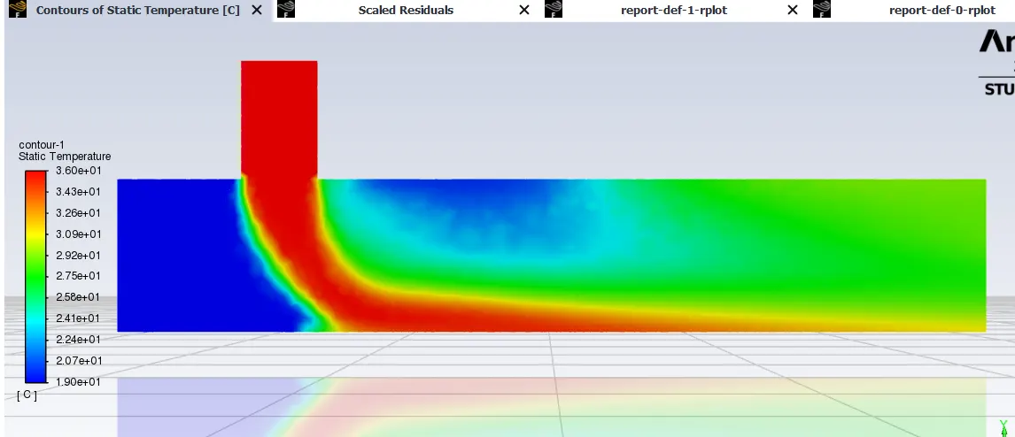
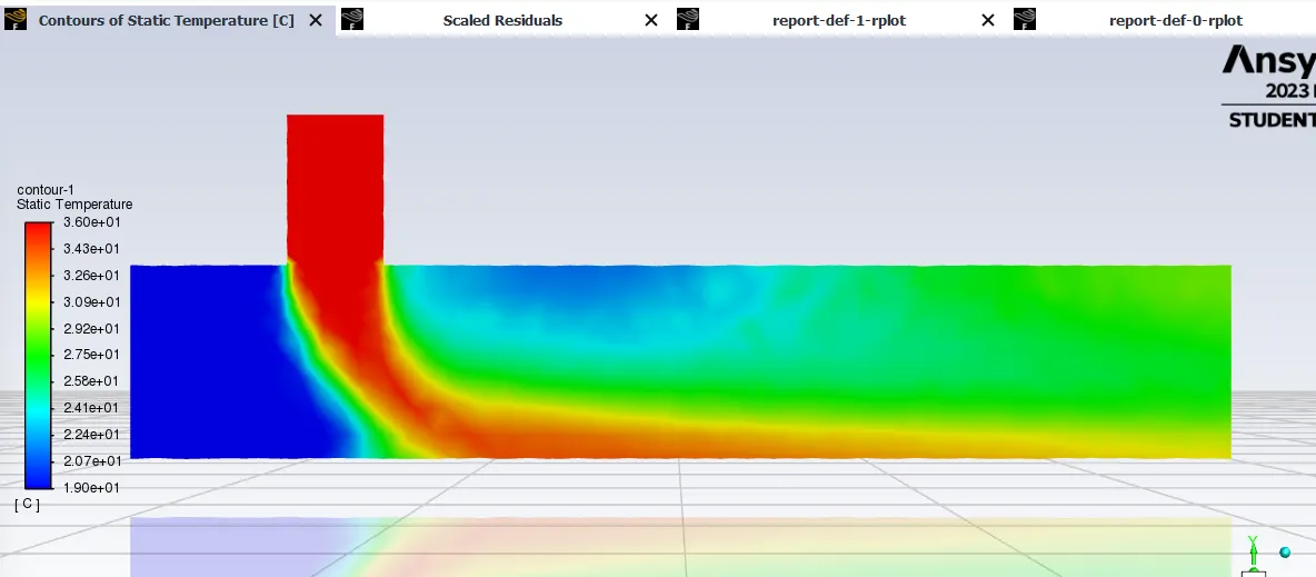
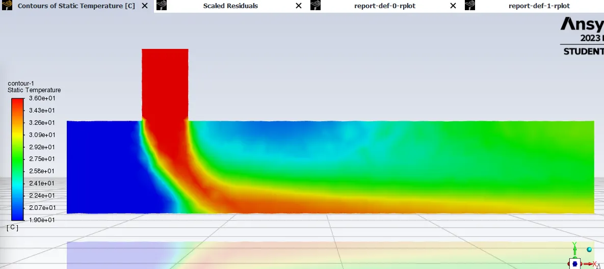
• here we performed the simulation for the case 1.1 with element size as 0.002, 0.005, 0.01, 0.02.
• As the element size decreases, number of elements (cell count) increases.
• velocity contour for element size = 0.002 m:
• 
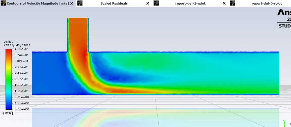
• velocity contour for element size = 0.005 m:
• 
• velocity contour for element size = 0.01 m :
• 
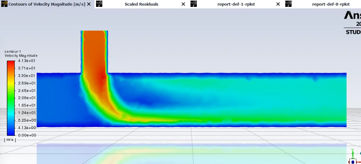
• velocity contour for element size = 0.02 m :
• 
• temperature contour for element size = 0.002 m :
• 
• temperature contour for element size = 0.005 m :
• 
• temperature contour for element size = 0.01 m :
• 
• temperature contour for element size = 0.02 m :
• 

Conclusion:

1. Conclusion of mesh independent study: 

• so from the mesh independent study, we can say that simulation results are dependent on the underlying mesh. As the element size decreases, number of mesh elements increases as mesh becomes more finer, and it results with fine simulation results.

2. Effect of length and momentum ratio on the results :

• As per the data collected from the simulation of flow through both short and long mixing tee's with same input data like minimum temperature, maximum temperature, velocity at inlet with hot air, velocity at other inlet with comparatively cold air, etc shows that if the length of tee is more, it will comparatively gives low average temperature at the outlet.
• If momentum ratio increases, the velocity of inlet through inlet-x increases, that results in decrease in average temperature at the outlet. This happens because, as the velocity of cold air increases, the amount of cold air increase in the mixture thus subsequently results in reducing the average temperature of mixture at the outlet.