Week 1- Mixing Tee

AIM:-

In this Challenge, we have to create two versions of the mixing tee. One of them is longer than the other.

So, we need to set up the steady state simulation to compare the mixing effectiveness when the hot inlet temperature is 36°C & the Cold inlet is at 19°C. And also we need to use the K-epsilon and K-omega SST model for the first case.

Case 1:- Short mixing tee with a hot inlet velocity of 3m/s and Momentum ratio of 2,4.

Case 2:- Long mixing tee with a hot inlet velocity of 3m/s and Momentum ratio of 2,4.

And also we have to compare the values through a table.

• cell count. 
• Average outlet temperature.
• Number of iterations for convergence.

INTRODUCTION:-

The mixing tee mixes the two fluids and analyzes the mixing phenomena so that it can help us improve the efficiency of the outlet temperature. so, In this Mixing tee simulation, our objective is to mix the two different fluent at different inlet stages of the temperature and velocity. Then we'll also need to analyze the two fluids mixing phenomena at the inside of the pipe and also we need to analyze the temperature of the outlet and also analyze the fluid flow of the outlet with the help of some physics models.

Applications:-

1. Air Conditioner system (A/C)
2. Petroleum industry. 

THEORY:-

• The T-Joints are important flow control devices we can find them in many areas. the T-joints are splint the flow and the angle between ∠ 90° degrees.

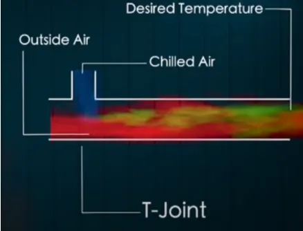
• For example:- The air conditioner system and the refrigeration system can provide the air at 10° degrees. but 10°C is too cold for me. so, I need to change the temperature to 25°C. For this kind of problem, the mixing tee is useful.
• So, I can have outside air in one of the inlets and I can have chill air in another inlet. Now by adjusting the flow rate of chilled air, I can get the desired temperature of the outlet of the mixing tee. which would be connected to the air-conditioned space.
• And this entire process is going to simulate using ansys. by using ansys work bench we can establish the workflow from SpaceClaim, seduo mesh, set fluent, and set CFD Post Process.
• The first thing I need to do is create a computation model so that is why we use ansys spae. We can see here the solid model. To capture the fluid volume there is a volume extraction utility in a space clam by selecting the respective edges.
• In this model there is a wet volume and solid volume. the wet volume is a volume that's occupied by a fluid. Then it's ready to create the computational mesh. we will use the ansys meshes. the mesh type is tetraheatel mesh with an inflution layer is captures the boundary layers.
• After checking the simulation quality and meshing matrics such as orthogonality and skewness. then we are ready to move a become fluent. ansys is used to set initial boundary conditions and numerics for this particular problem. And we are employing a steady-state solver in a sudo transient mode in this particular case.
• And we use as well as turbulence model after that we will set up convergence criteria. now since the simulating flow through a mixing tee, we need to measure the effectiveness of mixing.
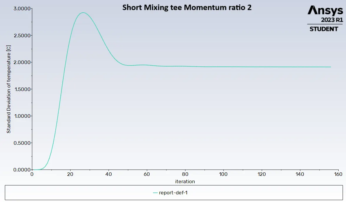
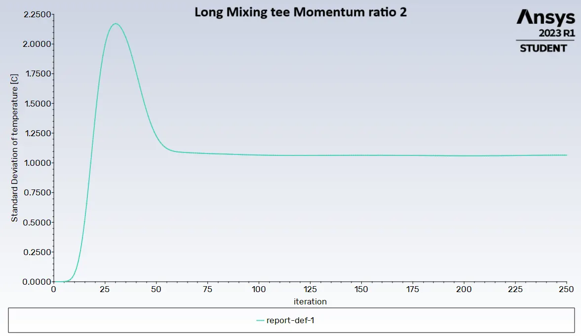
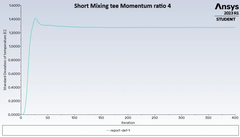
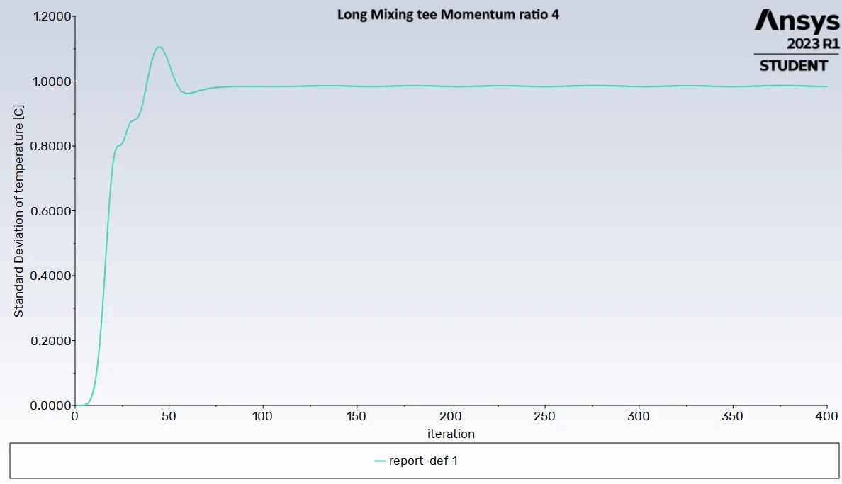
• And this is where the elementary statistics come to our rescue. We can calculate the standard deviation of the temperature at the outlet to measure the effectiveness of mixing. the high standard deviation means the mixing is bad. and the low standard deviation means that we have a pretty good mixing. 

ASSUMPTION:-

We need to find the Analytical value of the outlet Temperature and velocity.

1. For Analytical temperature output°c.

• To find the average outlet temperature we have to use the above formula. so, we need to find the Mass of the hot inlet (M_Ih), the Mass of the cold inlet (M_Ic), and the Mass of the outlet (M_o).
• So, to solve the M_Ih and M_Ic we need to use the law of conservation of mass flow rate can be used.
• The M_o is nothing but a M_Ih + M_Ic = M_o of  
• The law of conservation of mass flow rate is ρ.a.v
• (i.e) ρ= density is 1.28, a= area is [π/4(d²)], v= velocity.
• Now here the velocity varies according to the inlet-x and inlet-y and momentum ratio so for momentum ratio 2 we can use the velocity of X=3, Y=6, and for momentum ratio 4 we can use the velocity of X=3, Y=12.
• The Temperature of the hot inlet and the cold inlet also varies according to the momentum ratio if the momentum ratio is 2 the temperature is X=25°c, Y=10°c and if the momentum ratio is 4 the temperature is X=36°c, Y=19°c. 

       2. For Analytical velocity output m/sec.

• V_o or V₃=a₁.v₁ + a₂.v₂ / a₃
• To find the velocity of the outlet we can use the above formula. In that formula the a₁ a₂ a₃ = area is [π/4(d²)] and V_o or V₃ is the outlet of the velocity

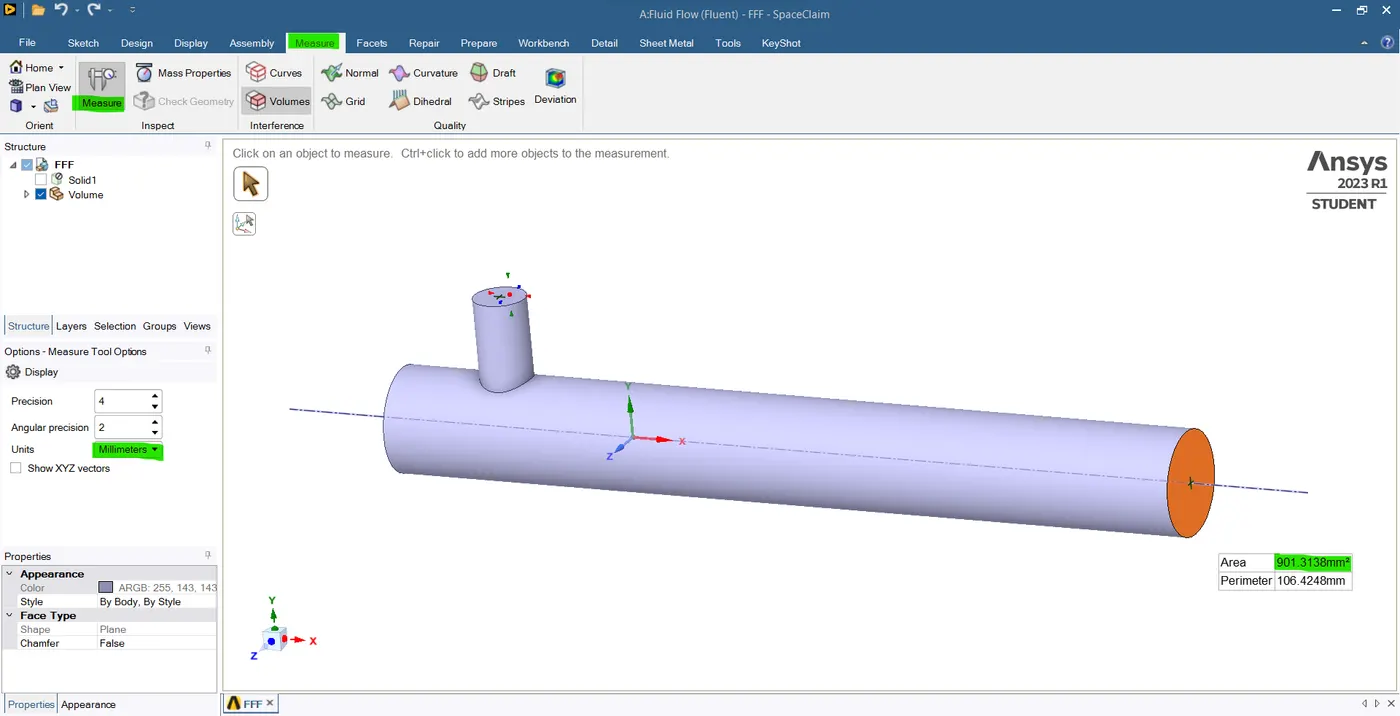
• To calculate the diameter in that area we have to use the Measure tool in that Geomentry section. so, just go to pre-processing of geomentry GUI and then go to the measure section and then select the measure option, and then change units as a Millimeter (mm).
• Now here the velocity V₁ V₂ V₃ varies according to the inlet-x and inlet-y and momentum ratio so for momentum ratio 2 we can use the velocity of X=3, Y=6, and for momentum ratio 4 we can use the velocity of X=3, Y=12. 

SOLVING & MODELLING APPROACHING:-

So, we have two mixing tees one is short and the other is a long mixing tee model. The two models are made in Solidworks software and we have SLDPRT File for importing it into the Ansys Fluent. we will use the steady-state solver to find out the temperature at the outlet with no heat transfer of the mixing tee.

we will be using k-epsilon and k-omega to solve this problem for the following cases:-

Case 1:- Short mixing tee with a hot inlet velocity of 3m/s and Momentum ratio of 2,4.

Case 2:- Long mixing tee with a hot inlet velocity of 3m/s and Momentum ratio of 2,4.

The momentum ratio is nothing but the ratio between the velocity of the cold fluid and the hot fluid.

Momentum ratio:- Vc / Vh 

Where Vc is the velocity of the cold fluid entering the pipe.

           Vh is the velocity of the hot fluid entering the pipe.

PREPROCESSING AND SOLVER SETTING:-

 For Analysing the temperature we need to import the geomentry of the Mixing Tee model into the ansys workbench for fluent flow analysis.

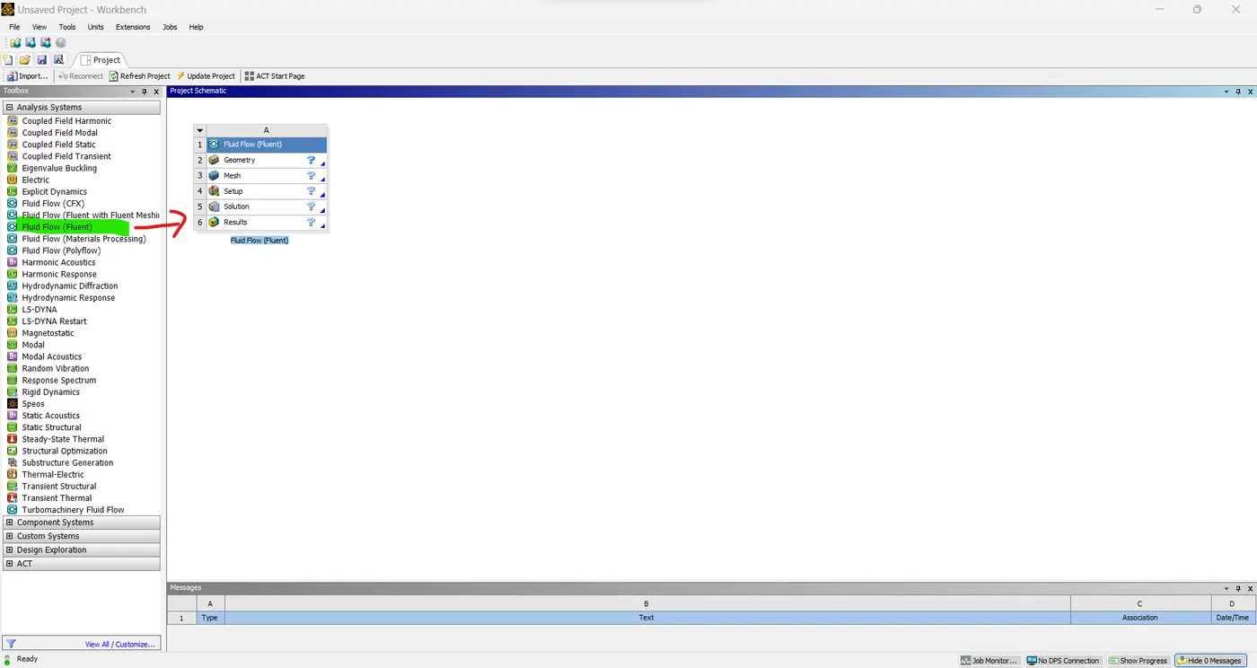
• First we need to download the model file and open that folder into the space claim. now we need to create a new fluid flow into the fluent system.

 

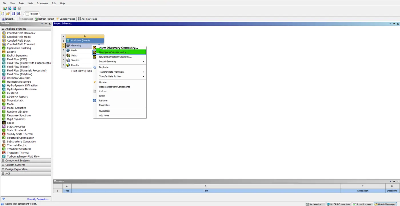
• go to geomentry -> new space claim -> import the model.

 

 

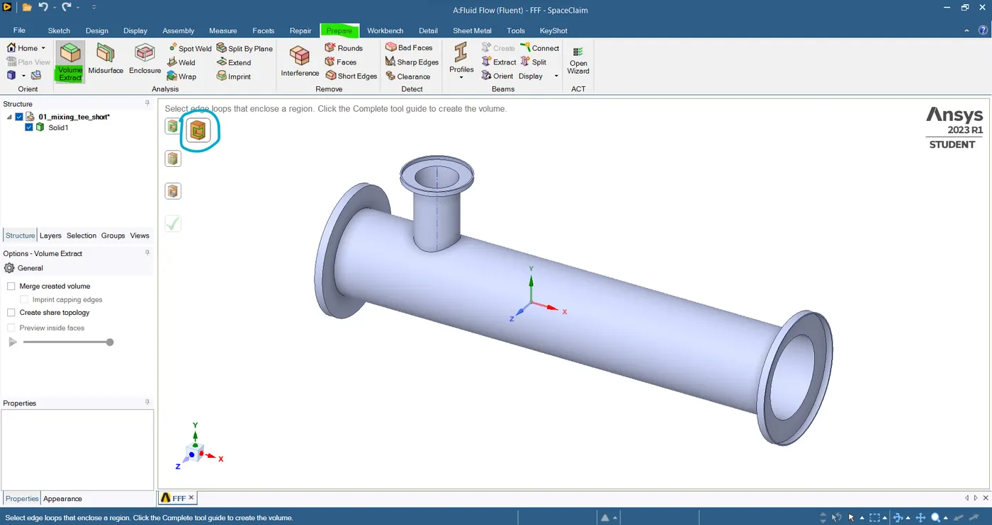
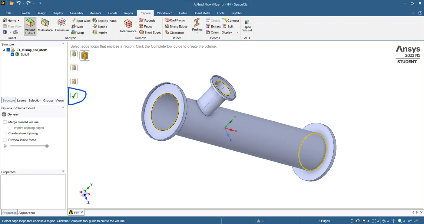
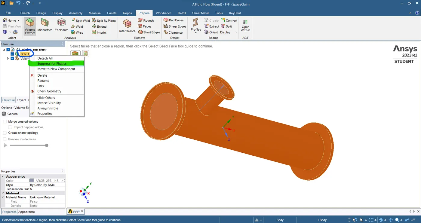
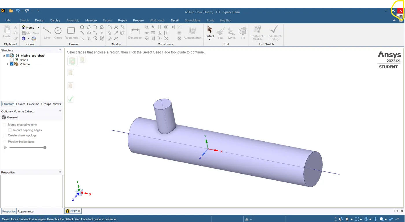
• click prepare -> select "volume extraction" -> select edge option -> select edge in the models -> select the solid and suppress for physics -> deselect the solid option -> close the geometry.

 

 

 

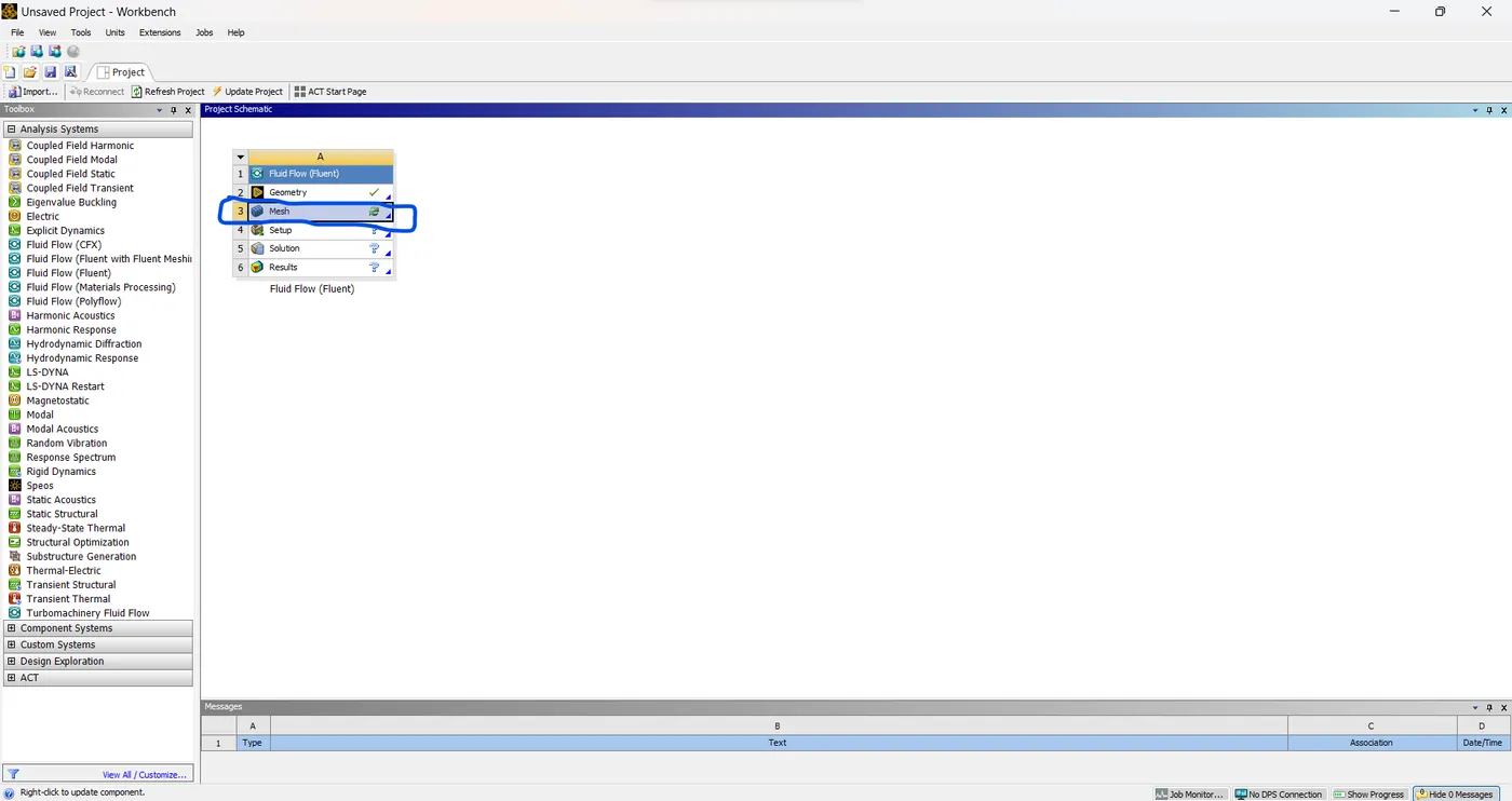
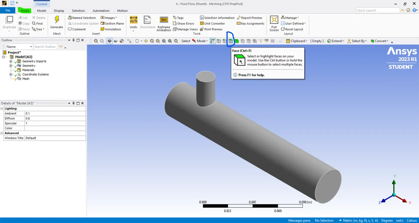
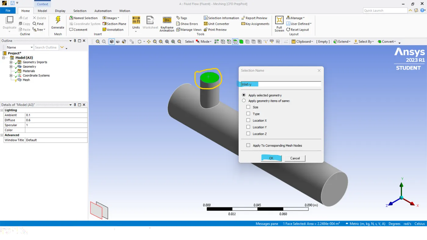
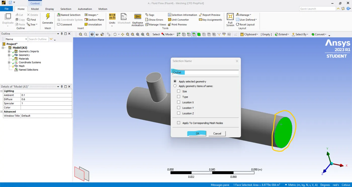
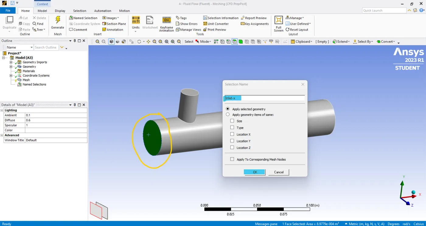
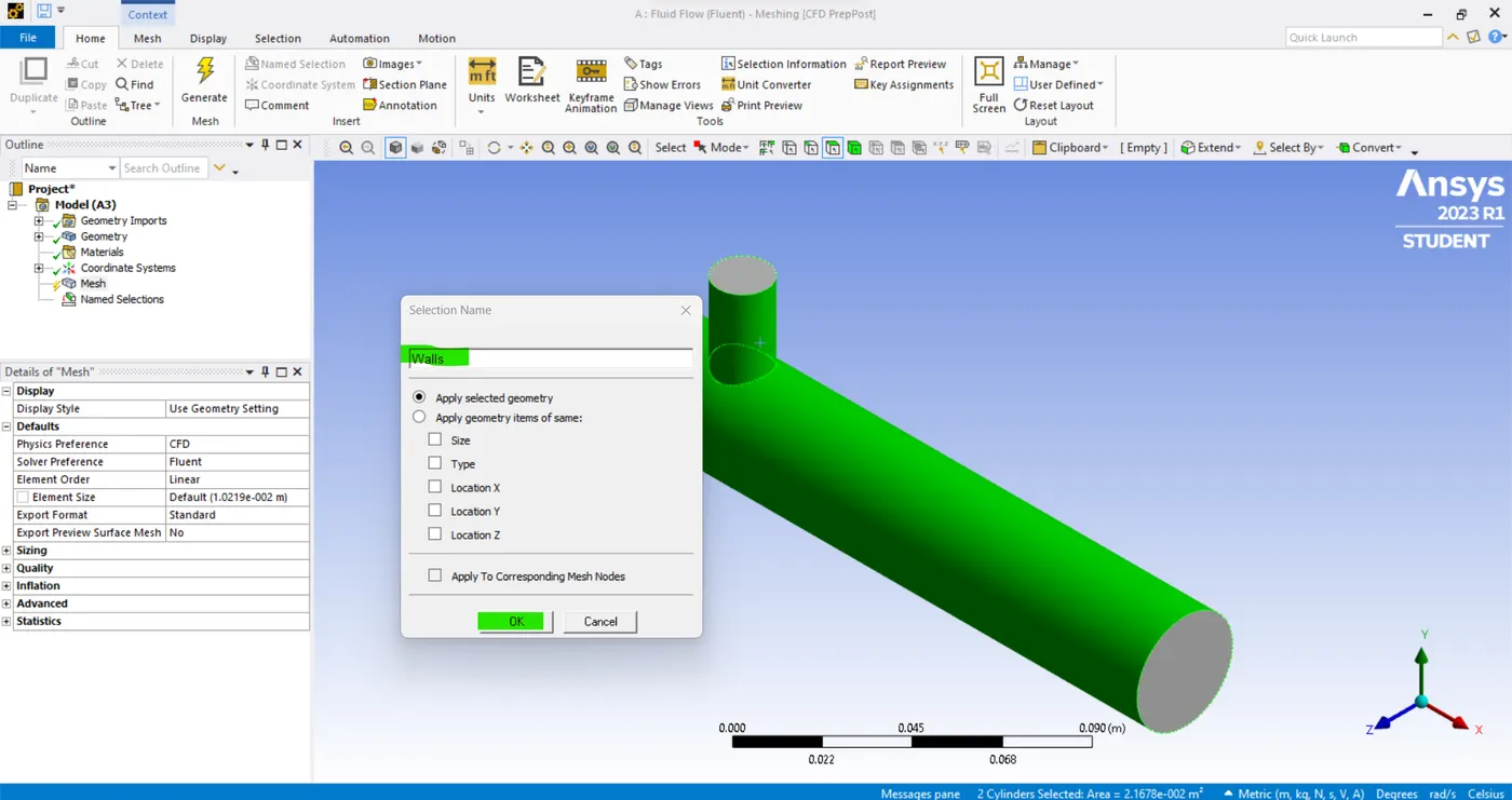
• now open the mesh mode -> Now we are going to name the boundary and we need to add the appropriate meshing -> Click Ctrl-F and select the face and "create named section" -> Enter the name as "inlet-y", "inlet-x", "walls".

 

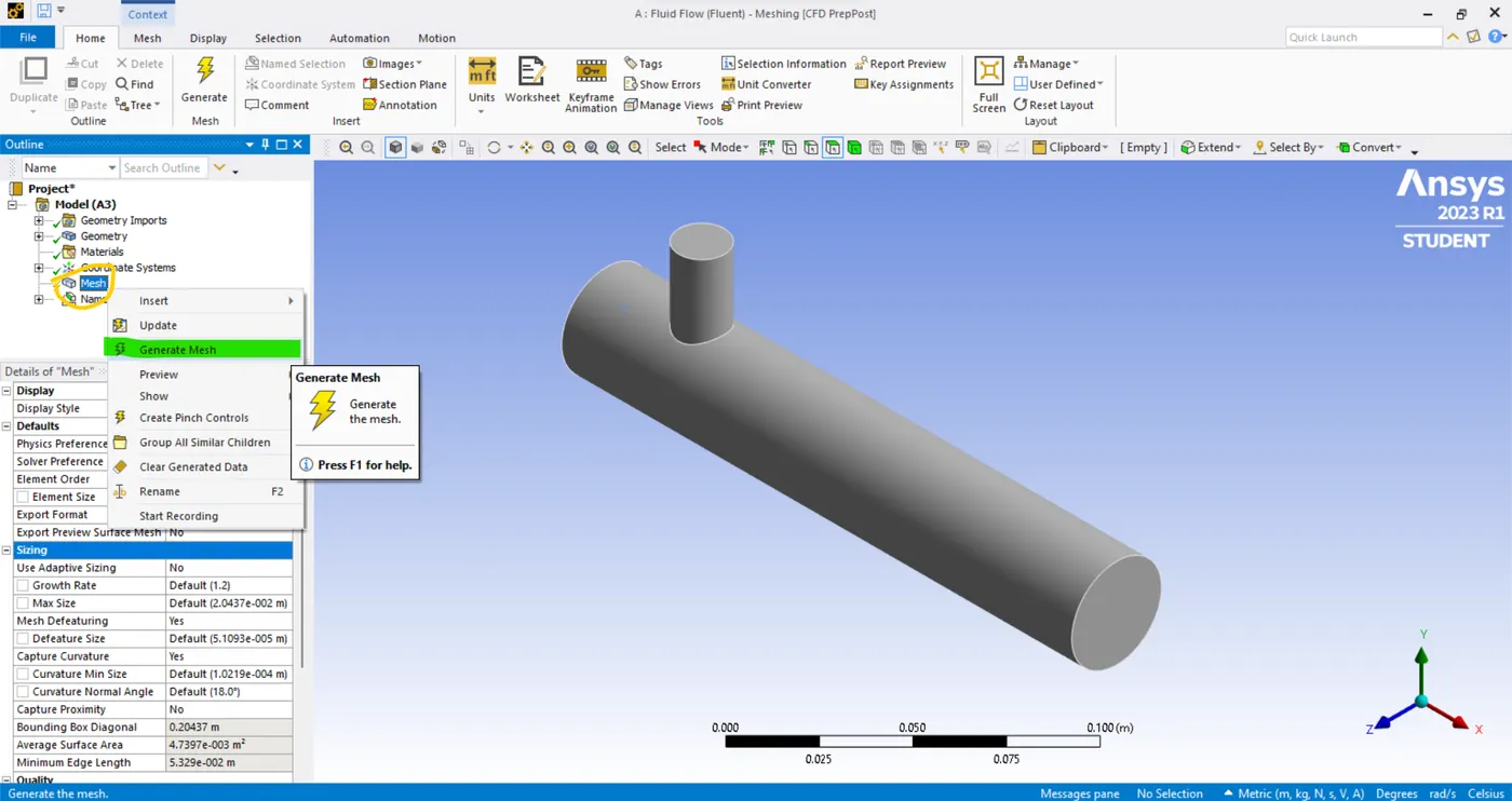
• Now select the mesh option -> and select the sizing in that sizing the value is already set it's predefined -> well the fluent use the boundary box.
• The boundary box is considered the geomentry. what's the smallest size box is fitted into the geomentry of the entire components. Based on that bounding box the mesh is created automatically. now right-click on mesh and select "generate mesh". now the mesh is generated automatically this is called a computational mesh.

 

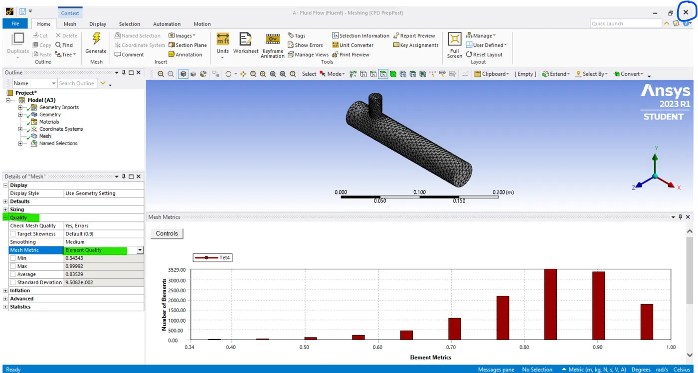
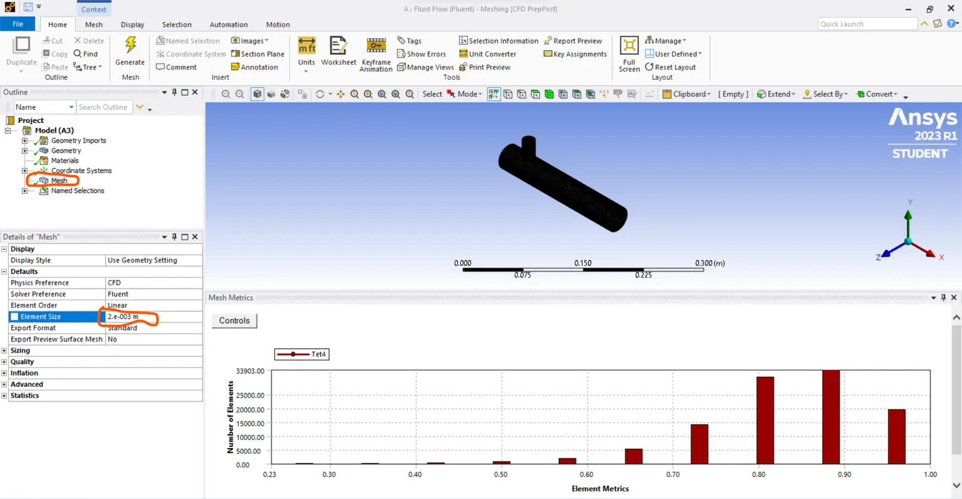
• Now we need to check the quality of the mesh. so, select the quality section on the right side -> and change the mesh matrix into element quality -> after now the histogram graph chart appears which is the mesh quality.
• Before understanding the team in the quality we need to know the finite volume discretization how the flexes are completed and what type of interpolation scheme is being used. To understand the quality of the mesh we must know about the interpolation scheme aspect ratio skewness and orthogonality.
• Just we need to make sure the element quality is not below 50%.

 

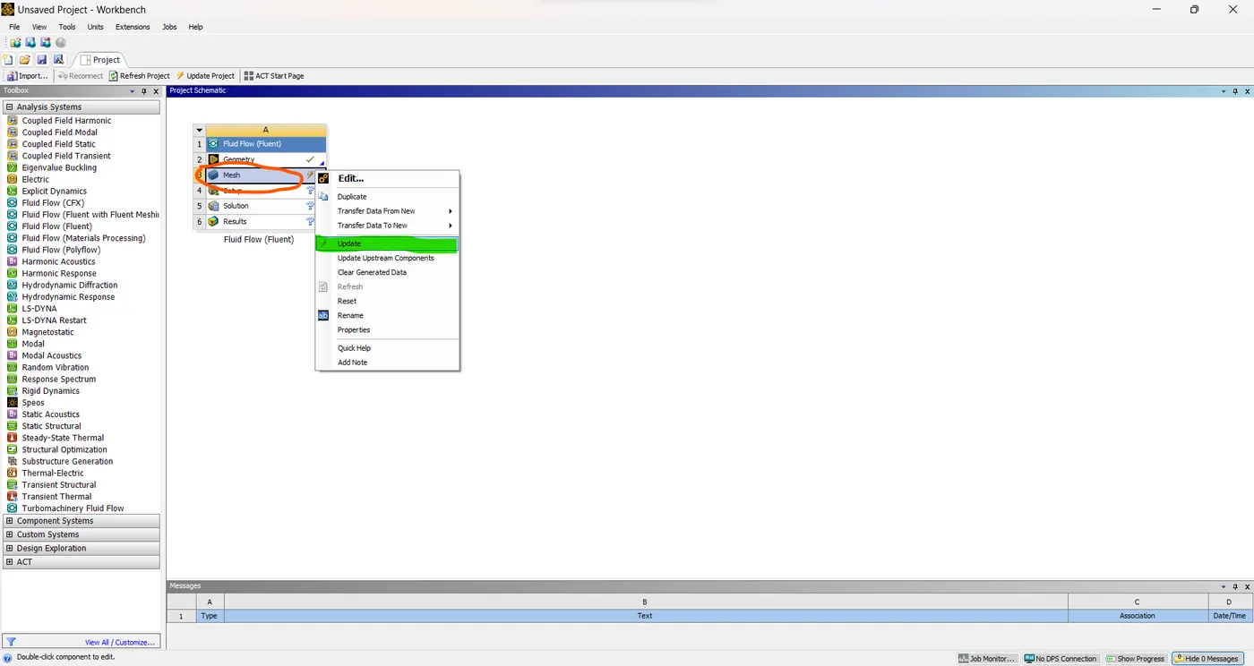
• Now close the mesh GUI and open the setup GUI -> In that select the parallel option enter the value as 4 and click "ok" -> If not the geometry is loaded in the setup GUI right-click the setup and click update. 

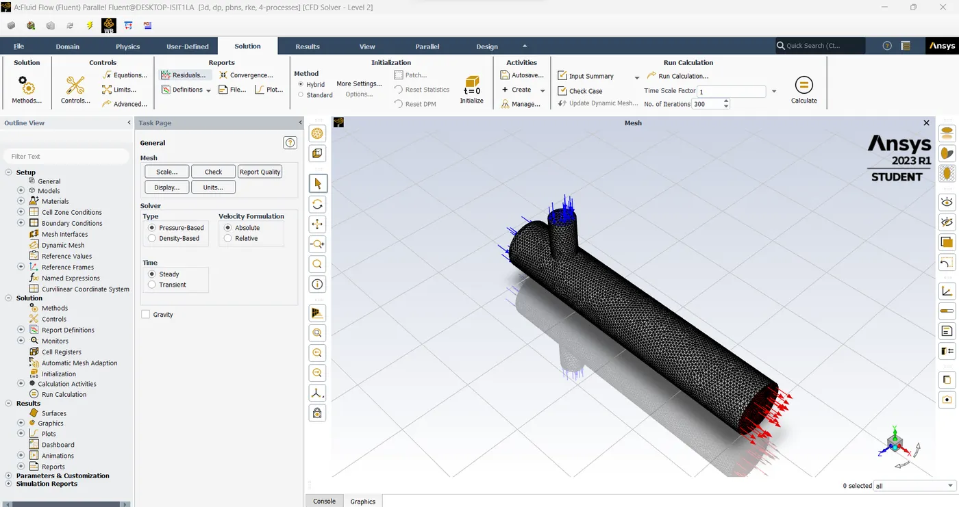
• In that select the setting up physics select the steady state in time select the pressure-based solver in the time and select the absolute in the velocity formulation. and now select the viscous model in that we need to set the viscous model in this way for how the turbulence is captured in my model.

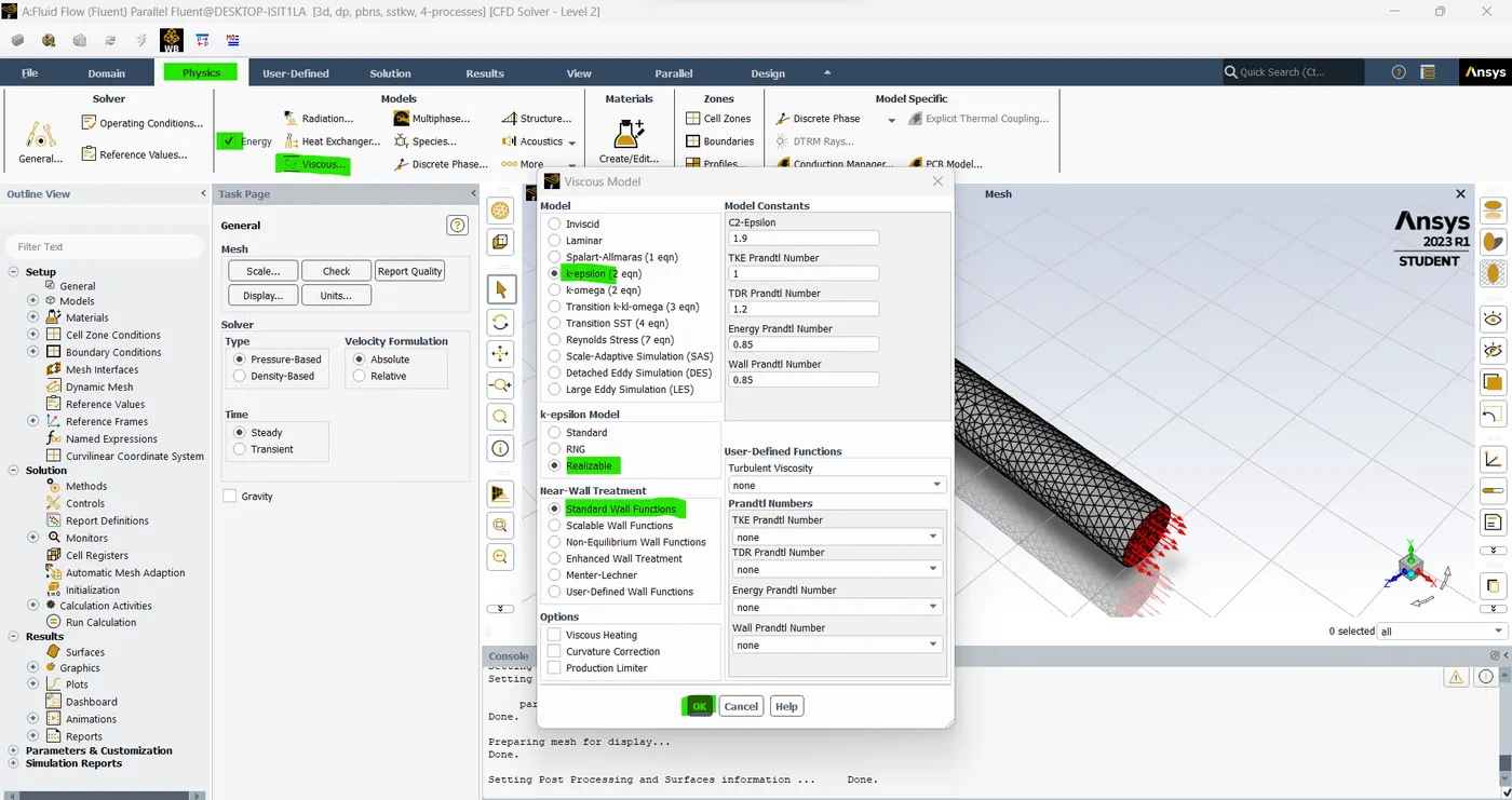
• The K-epsilon and K-Omega are called as Rans-based turbulence model or rentals-based turbulence model. Now we are going to add the material. so, click the create & edit in the setting up physics option. so, in that the air is the working fluid.

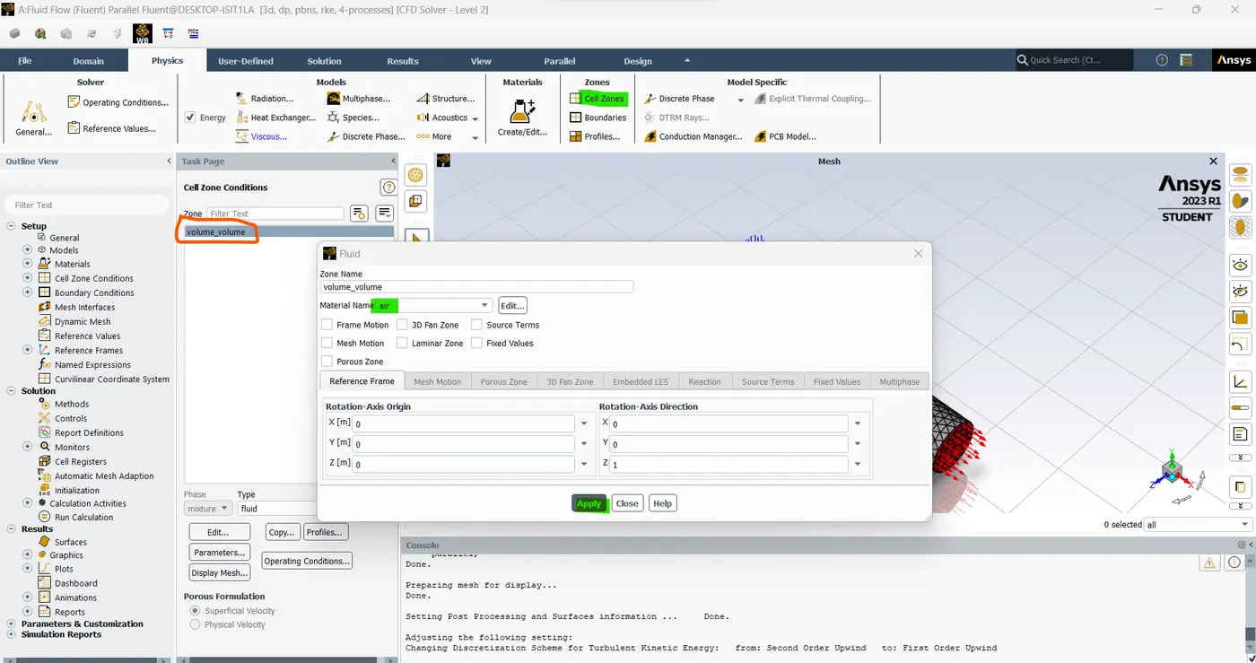
• Now go to zones select the cell zones select our volume regions and click the edit option In that option there is air is working fluently and click apply ok.

 

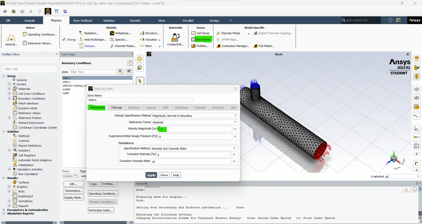
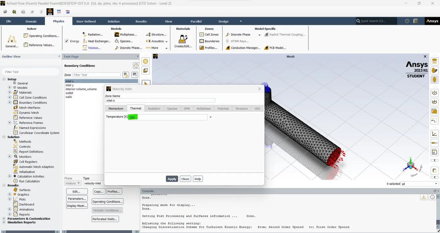
• Now go to the boundaries option select the cell zones select our volume regions and click the edit option In that option there is air as a working fluid and click apply ok.
• Now go to the boundary option and select the inlet-x and the type is automatically changed to velocity inlet. so, now click the inlet-x and click edit The velocity magnitude is 3m/s and the thermal is 300 Kelvin, and click ok.

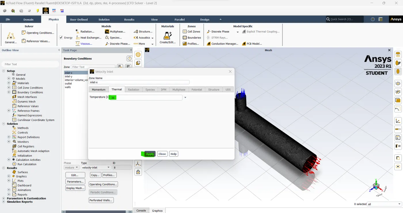
• We need to change the units of the temperature. so, go to setting up a domain and select units and in that tab select temperature as a Celsius and click apply ok.
• Now again go to inlet-x and go to thermal Now the Kelvin is converted into Celsius for the temperature and enters the value of 36°C. 

 

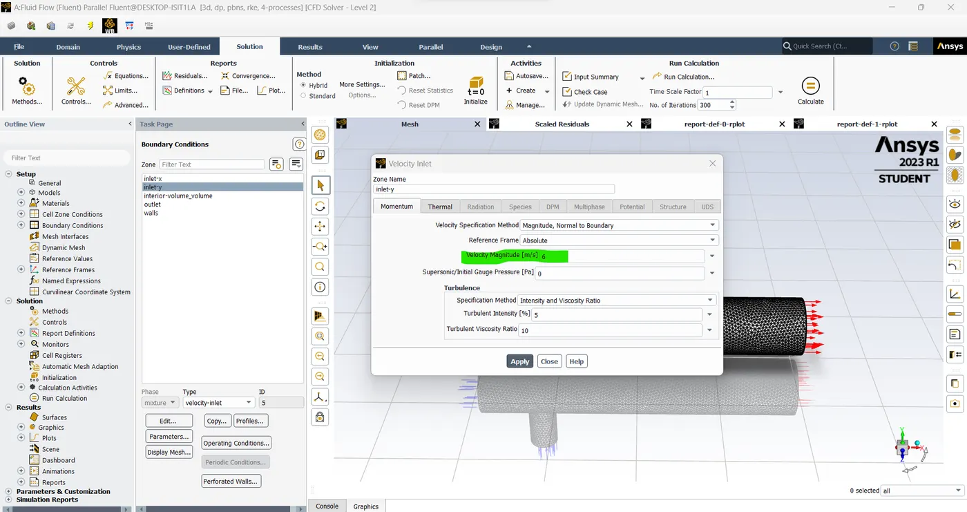
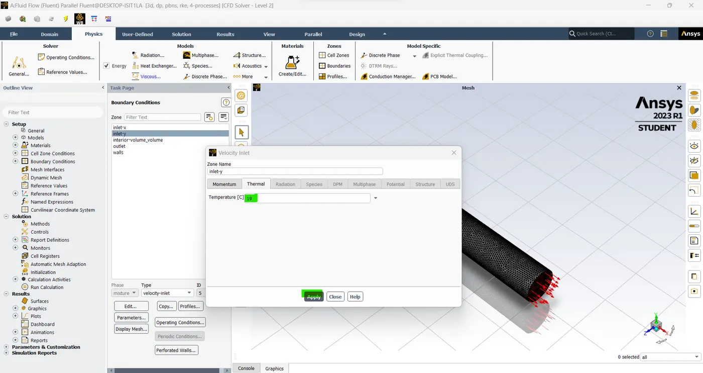
• the inlet-y viscosity is 6 m/s and the temperature 19°C.

 

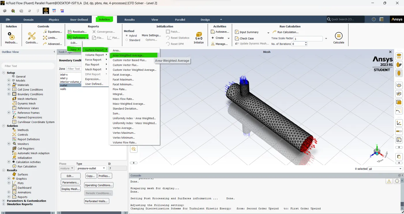
•  So, now we need to monitor the outlet of the velocity. so, we need to set the option easily. Just go to the "solution" section and click definition and in that option, we need to select new -> surface report -> "Area Weight Average".
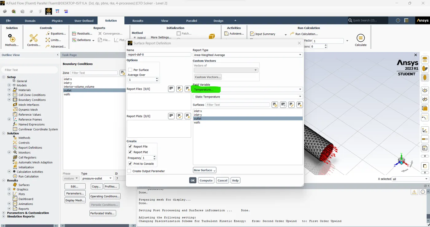
• Now select the field variable as a "temperature". select the outlet enable the report file and plot and click "OK". 

 

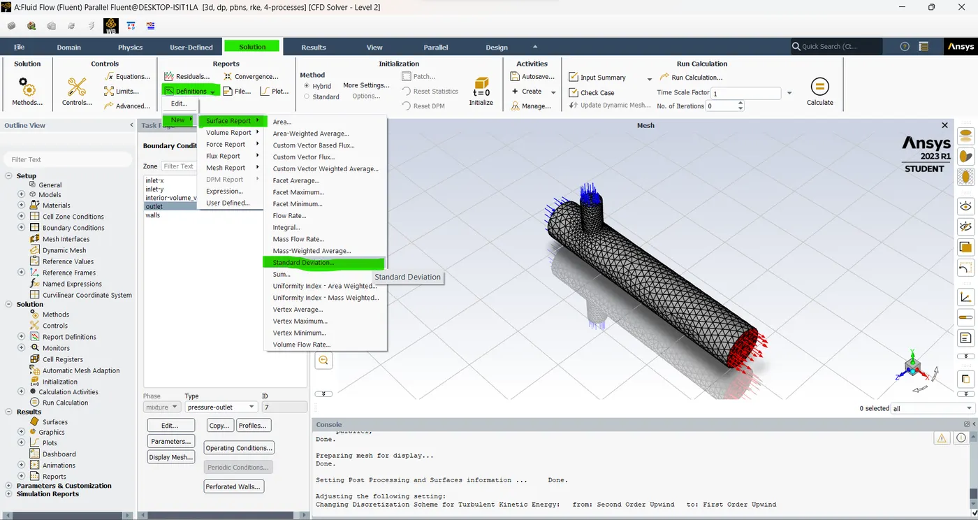
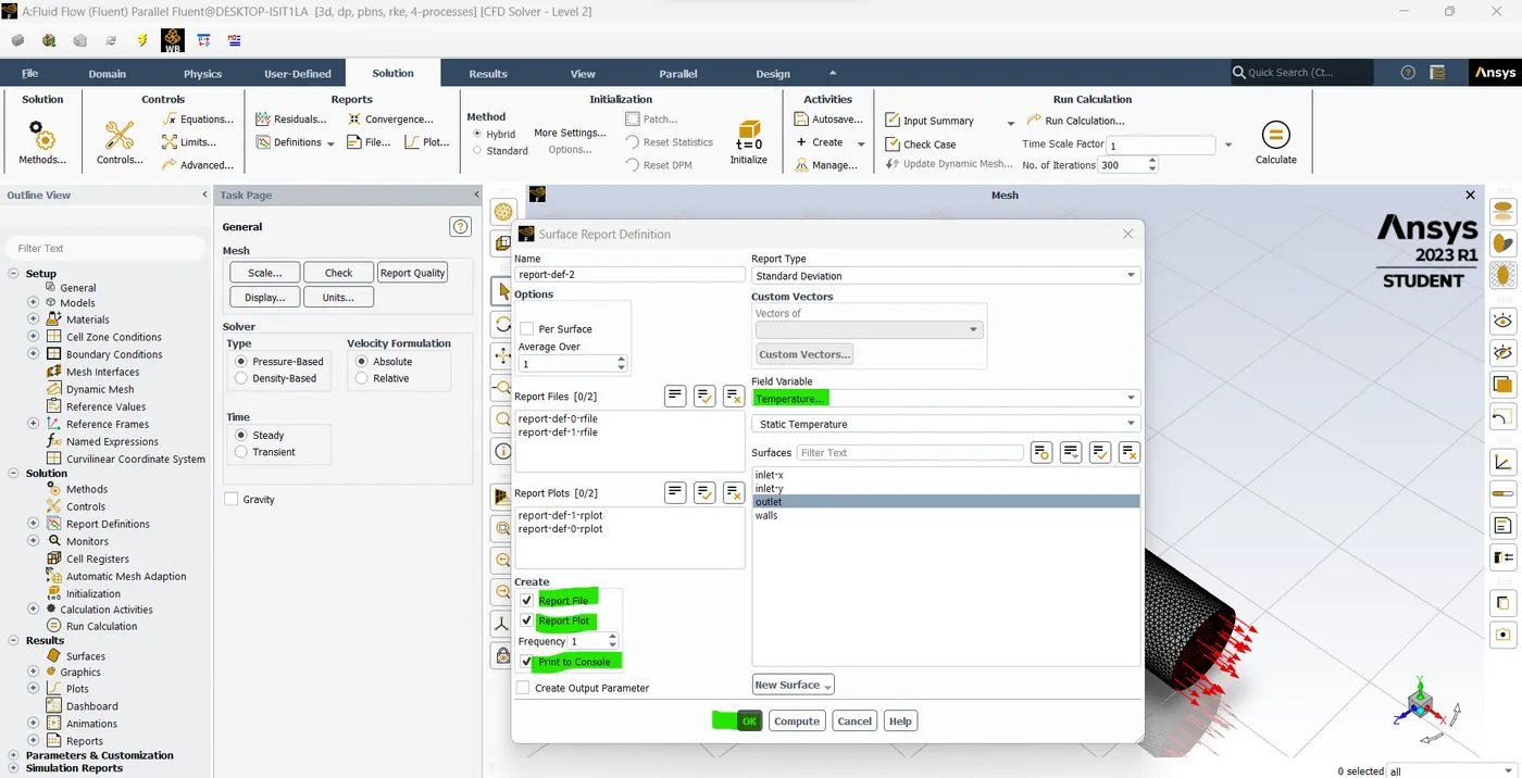
• To understand the mixing of the two fluids we need to create a second report as a standard deviation. so, click new -> surface report -> standard deviation -> in that table select temperature and outlet and report file and plot then click apply ok.
• Now once set all the initial condition boundary conditions and material properties the next thing we need to do is initialize the solution. 
• So, we need to set the boundary condition for the outlet where the gauge pressure is 0. It has been developed already. so, click ok.

 

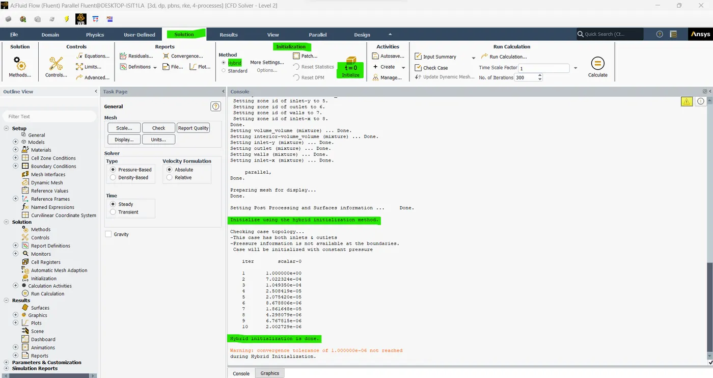
• Now we need to initialize the flow for that go to solving go to initializing click hybrid and click t=0 initializing. now the 10 hydration is completed.

 

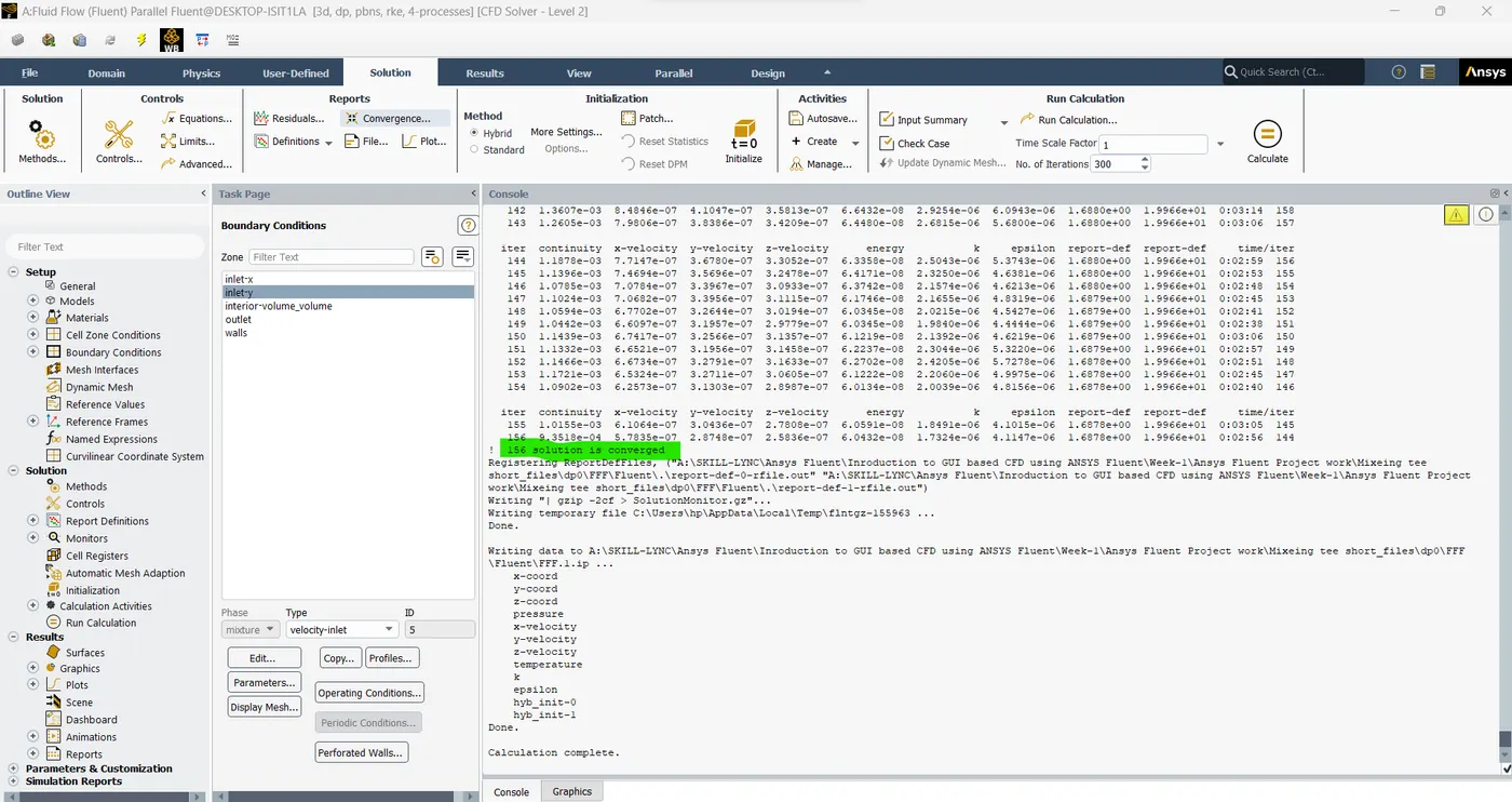
• Now I entered 150 in no.of Interaction in the run calculation and clicked calculate.

 

 

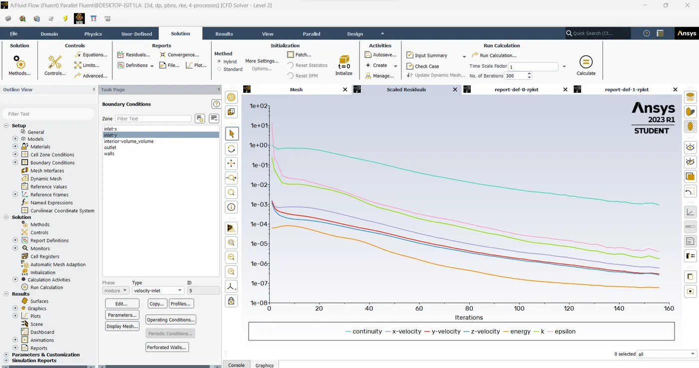
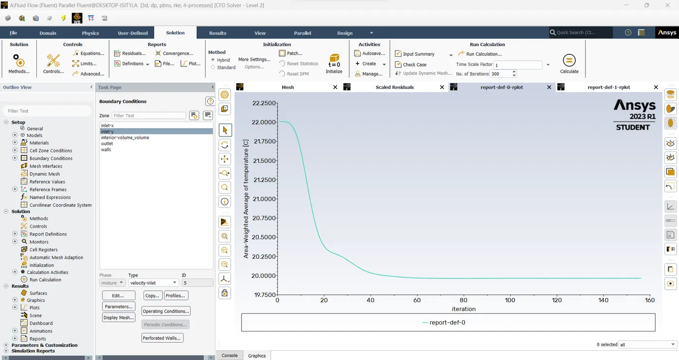
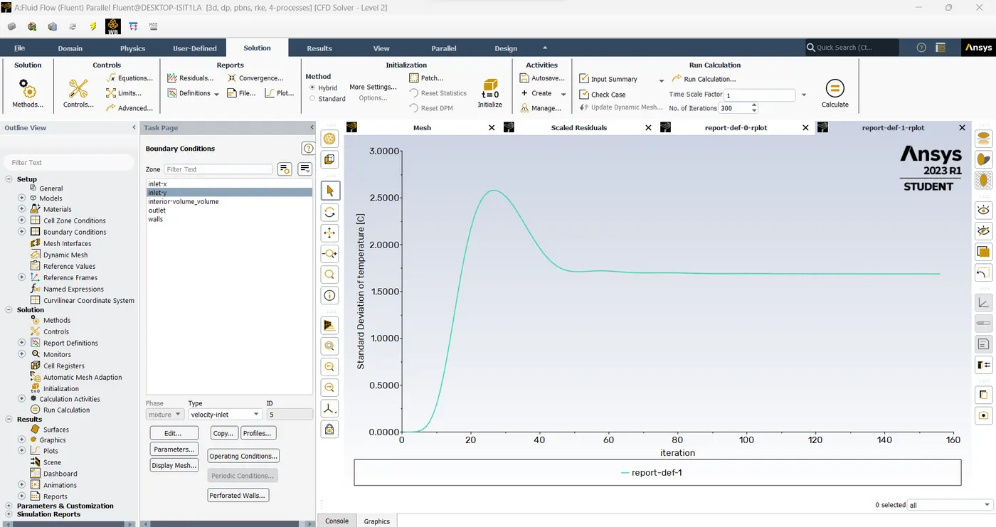
• Now, our standard deviation average weighted area, and residual have reached the steady state condition. but to get the complete steady-state condition we need to run a few more iterations. so, change the value from 150 to 300 iterations in the calculation section and click calculate.
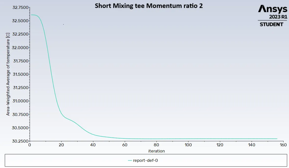
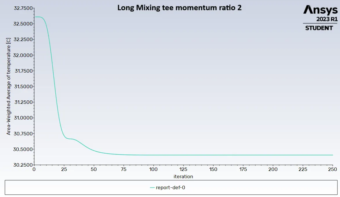
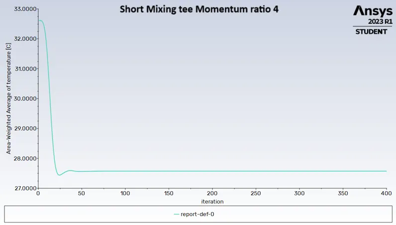
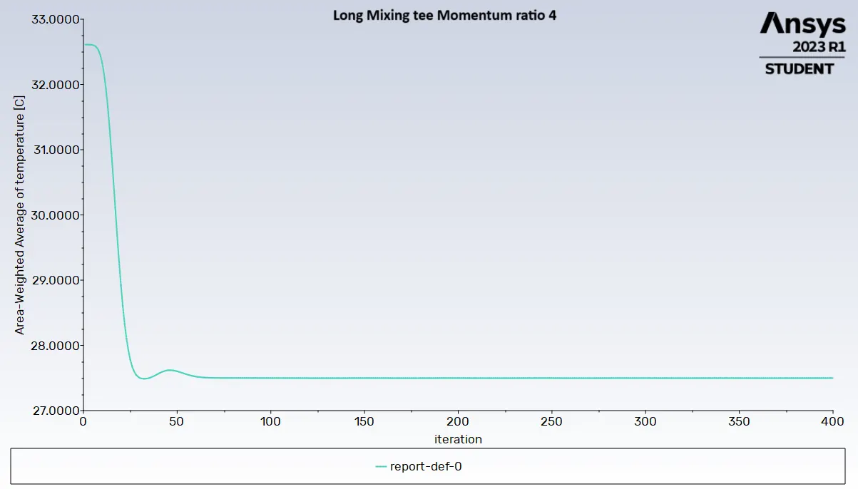
• Now our mixing tee graph has reached the completed steady state condition we can see that in the graph section. so, the solution is converged.

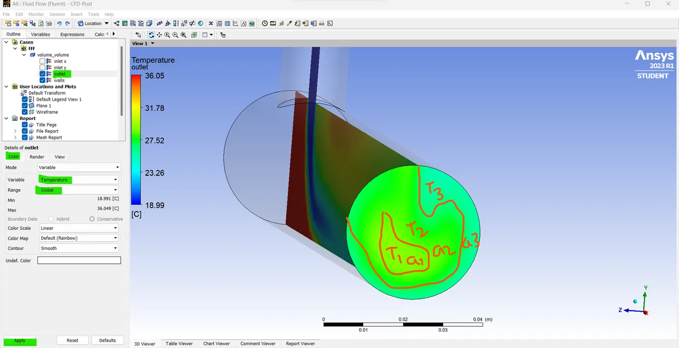
• In this simulation we are using "Area weighted Average" for monitoring an outlet temperature. we can see in the above image that there is no uniform outlet temperature distribution. we can see there is three different temperature and area occupied in that outlet contour plot. for this kind of outlet, we are using this Area Weighted Average to calculate the outlet temperature.
• Area Weighted Average = T1.A1+T2.A2+T3.A3 / (A1+A2+A3) 
• So, using this above formula the area-weighted average can be calculated automatically by the Ansys Software. 

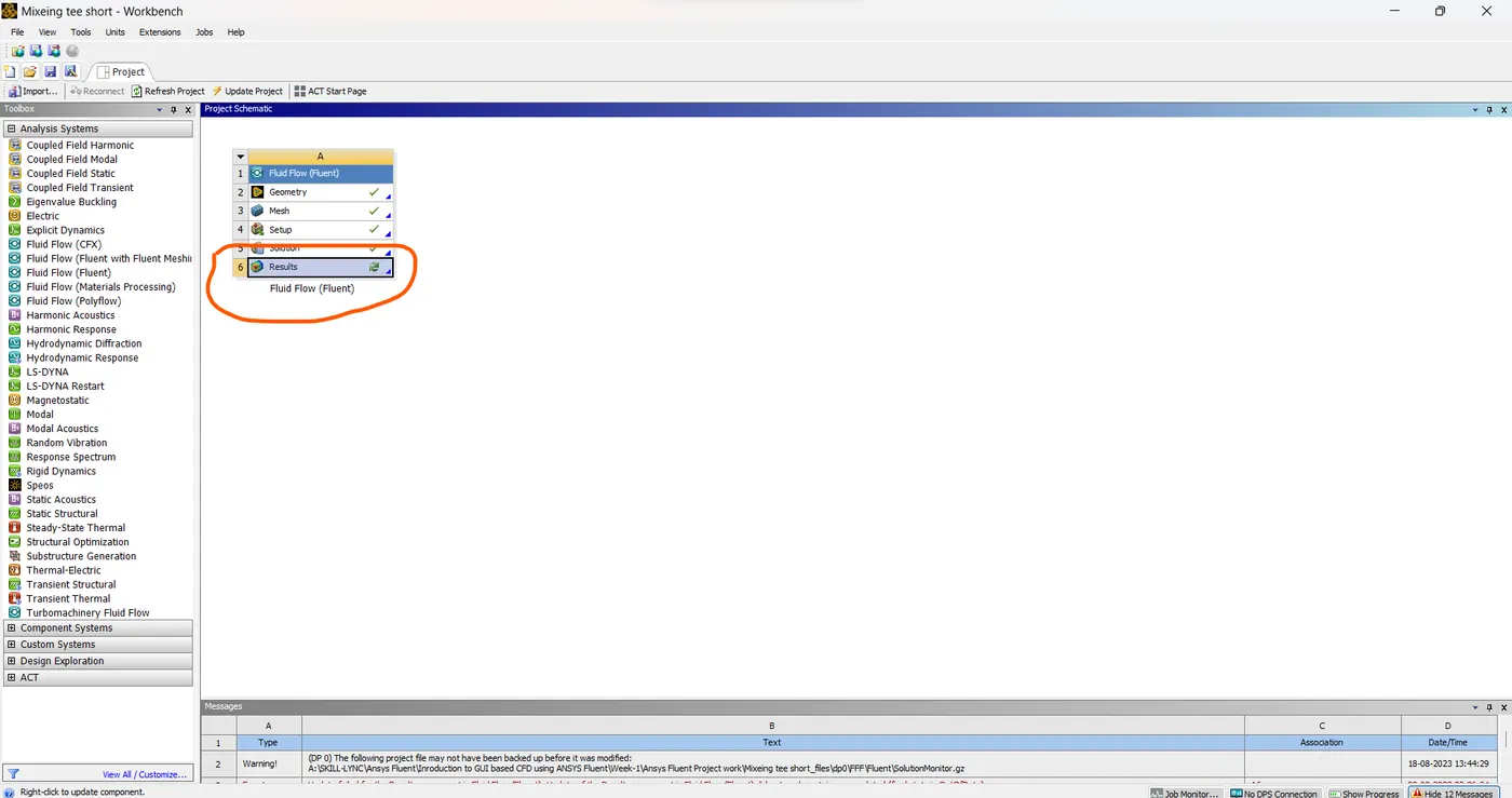
• So with our simulation having been completed now we need to post-process our result so, go back to our workbench and double-click the result Before doing this, close the fluent otherwise we will face some licensing issues.

 

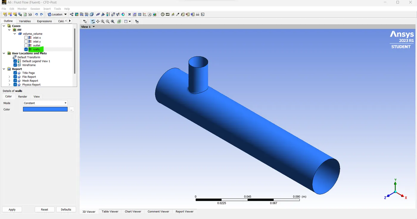
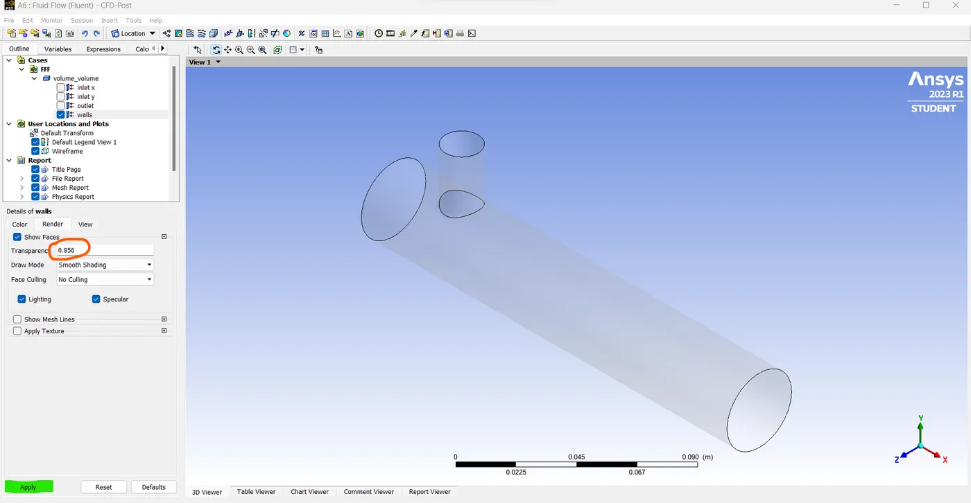
• So, after opening the result GUI. now enable the wall by clicking the walls in the "volume" in the volume section. so, double-click the walls and click render now to change the transparency so, By changing the transparency only we can see the amount of velocity inlet-y,x. so apply some transparency then only we can see the velocity and pressure distribution.

   

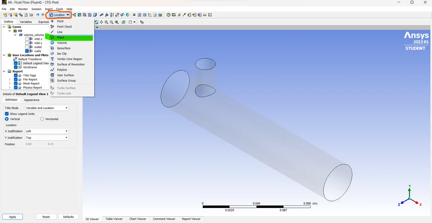
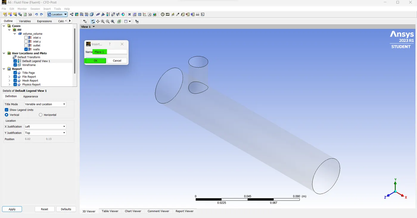
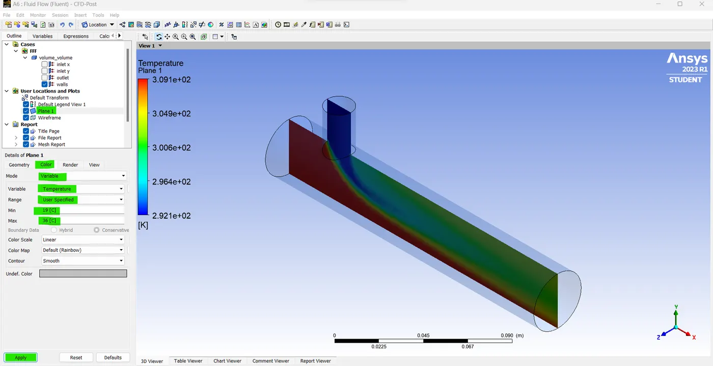
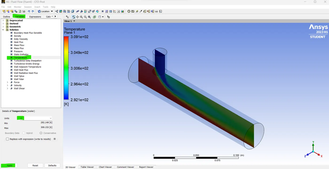
• go to insert -> location -> plane -> plane 1 and click apply. goto walls -> double click walls -> colours -> change the colour to white.
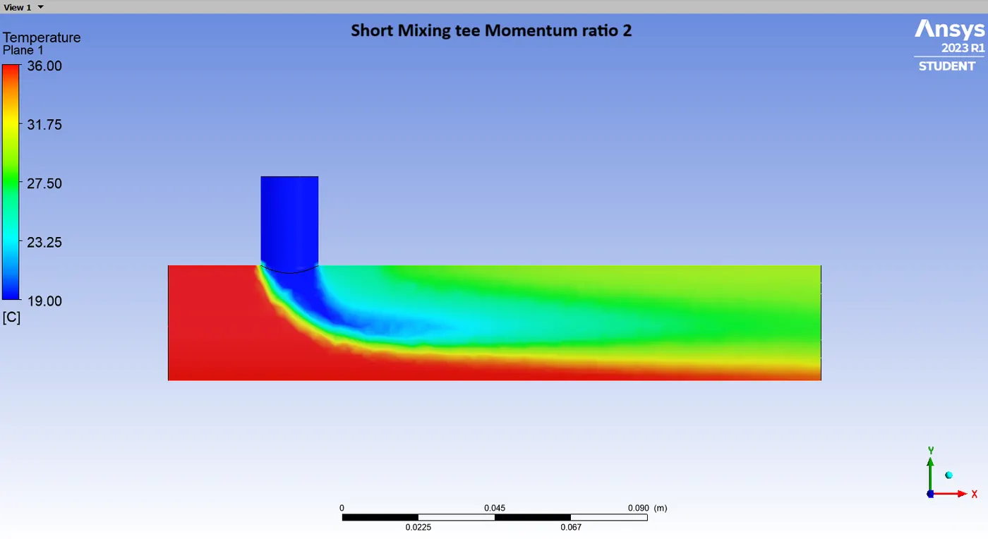
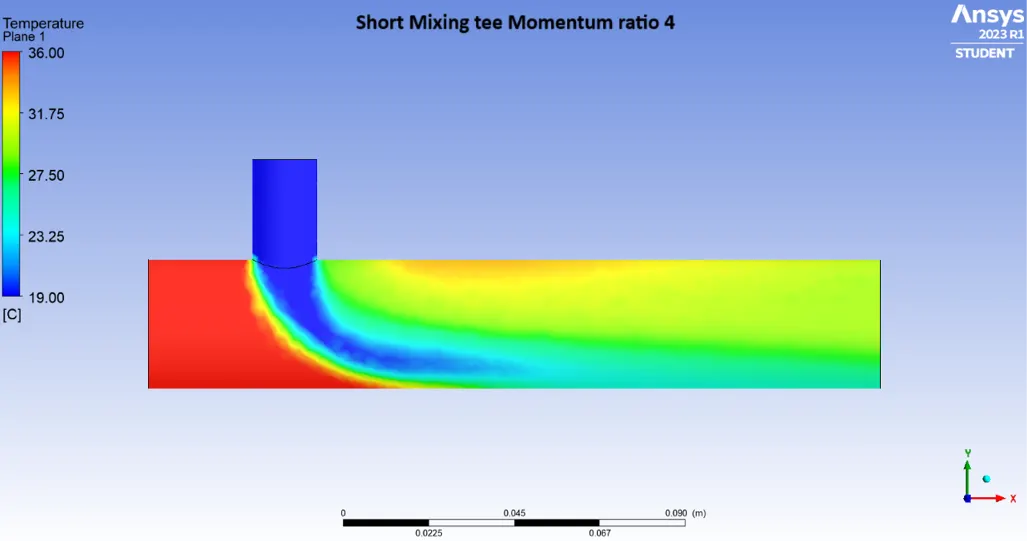
• The plane is created in the location and plots. so, double click plane 1-> color -> select the mode as available -> the variable as a temperature and go to range -> select user specified. now enter the value in minimum as 19°C and maximum as 36°C and click apply now the temperature is set.

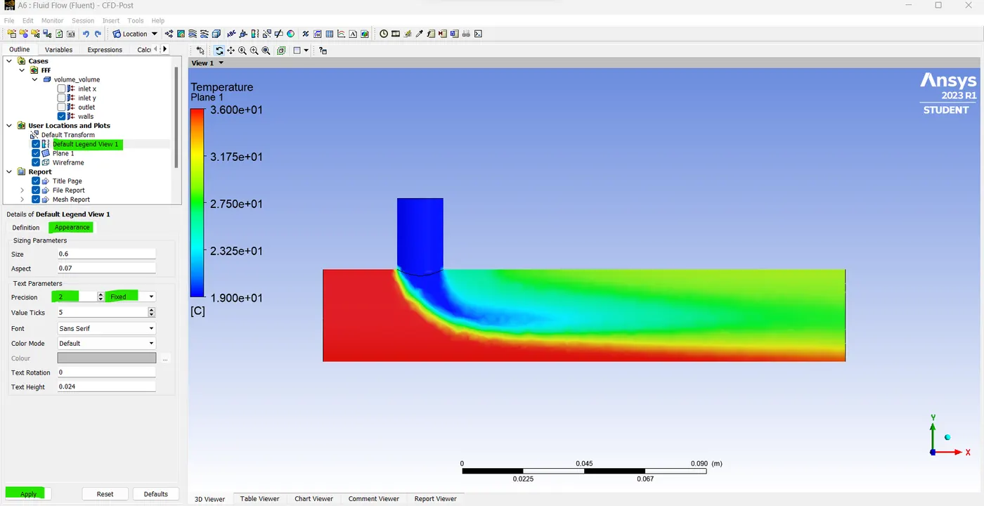
• Now double click the default legend view and go to appearance -> change parameter precision as a fixed and enter the value as 2. Now our temperature indication is fixed correctly.
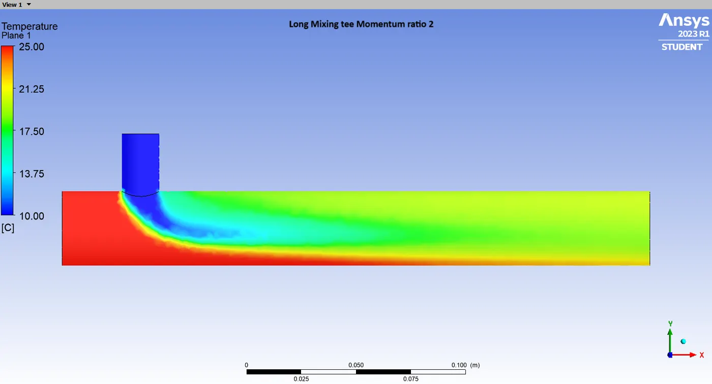
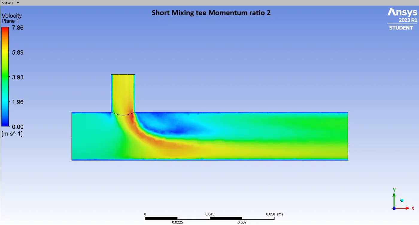
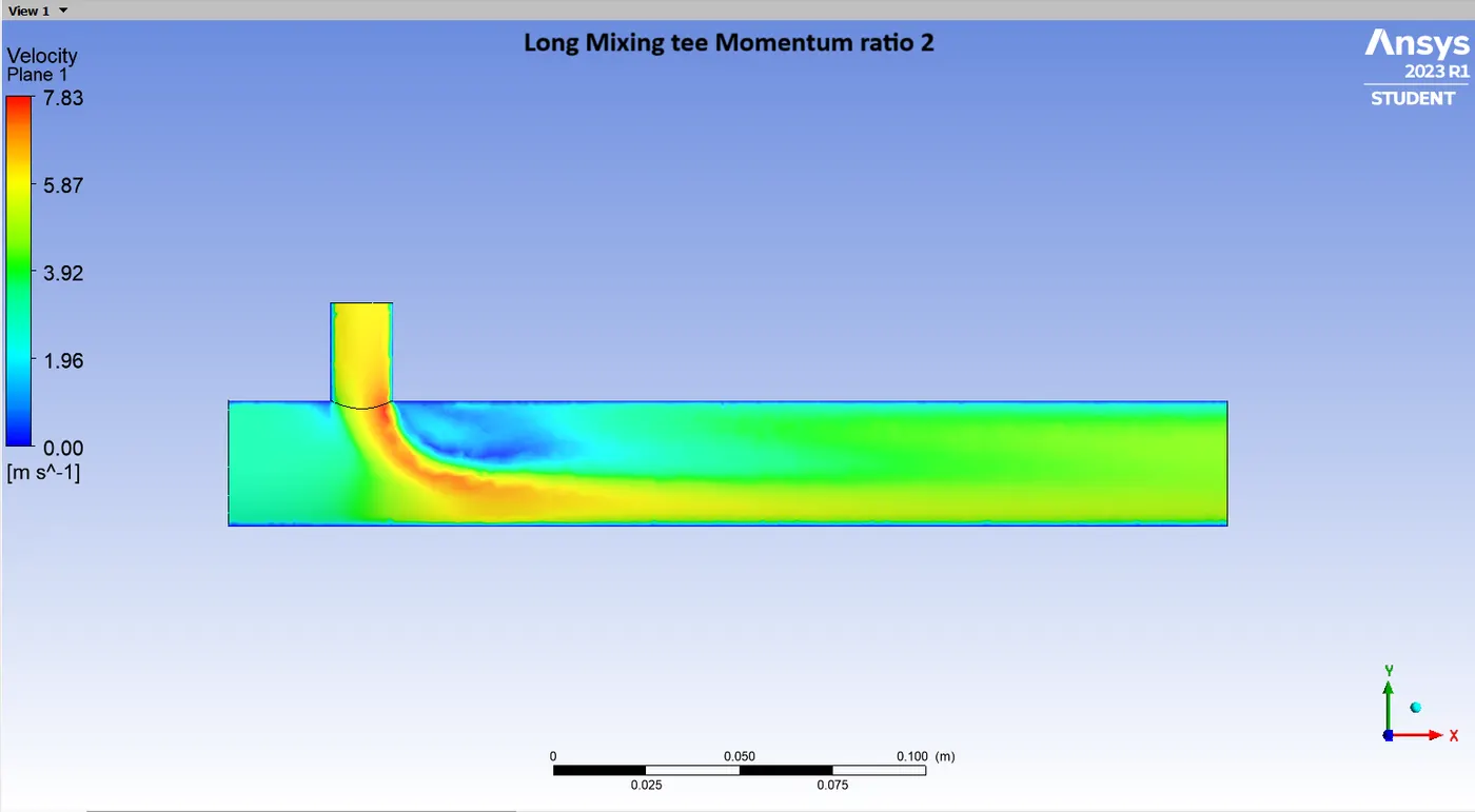
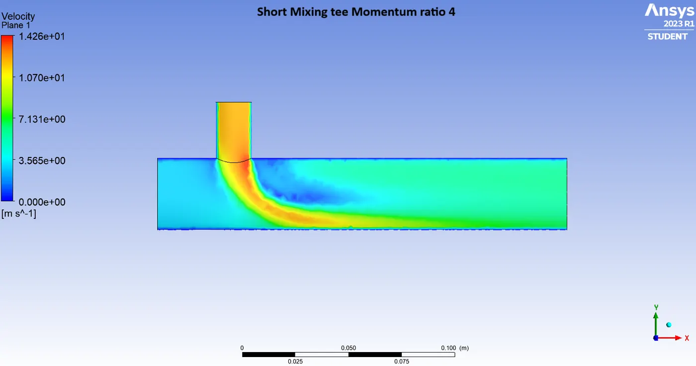
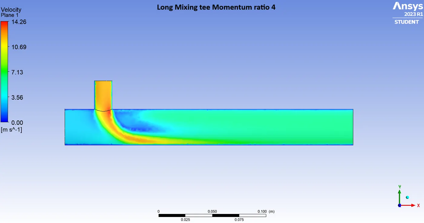
• So, here the mixing process is primarily determined by the velocity of the incoming jet and also we can use the different Moment Ratios. so, as you can see the cold inlet is 6 and the hot inlet is 3. So it depends on how we define the momentum ratio. we are examining the effect of the mixing process.

 

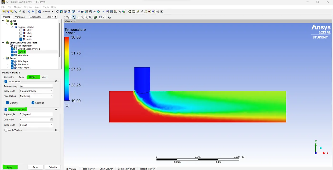
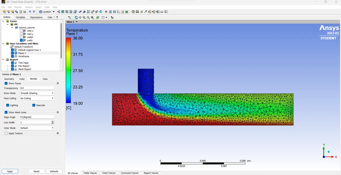
• So, in our model, the two-income inlet meeting area looks quite defused. so go to plain 1-> in that go to render -> enable the show mesh line.

   

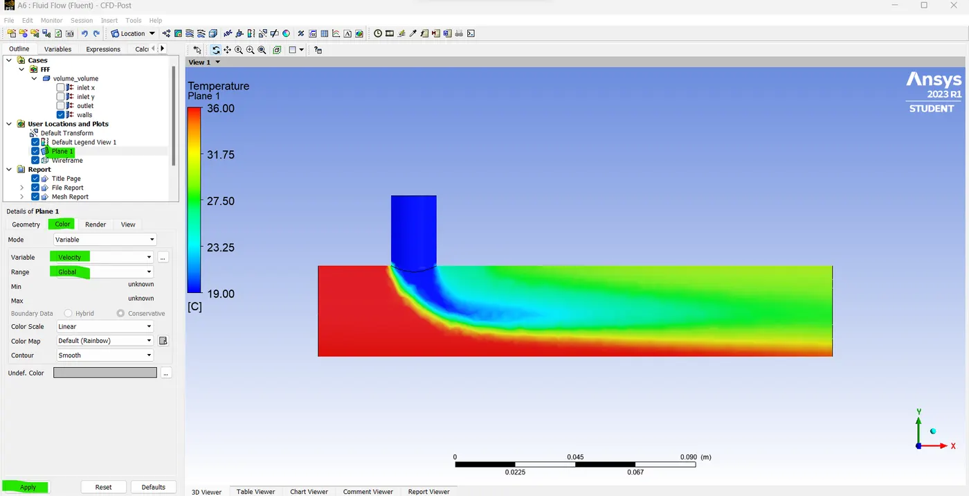
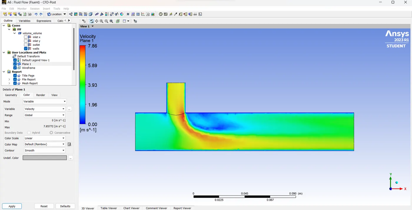
• To visualize the velocity in this mixing tee we need to change some options First go to plain 1 -> change the variable from the temperature into velocity as well as change the Range from the user-specified into global and then click apply.

   

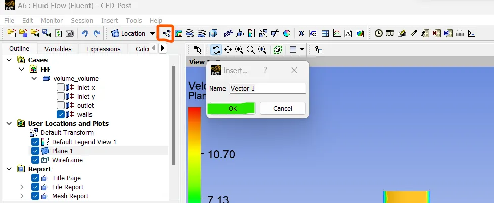
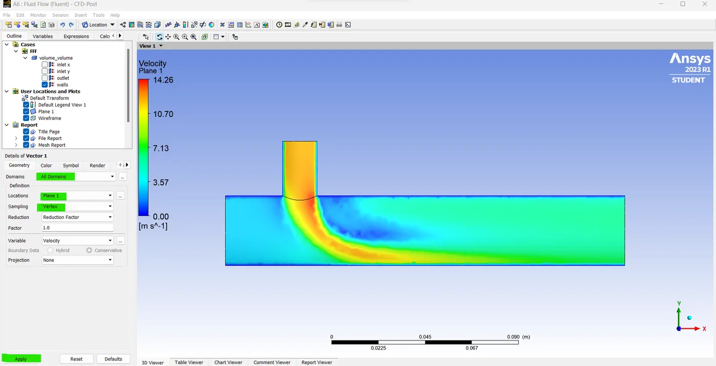
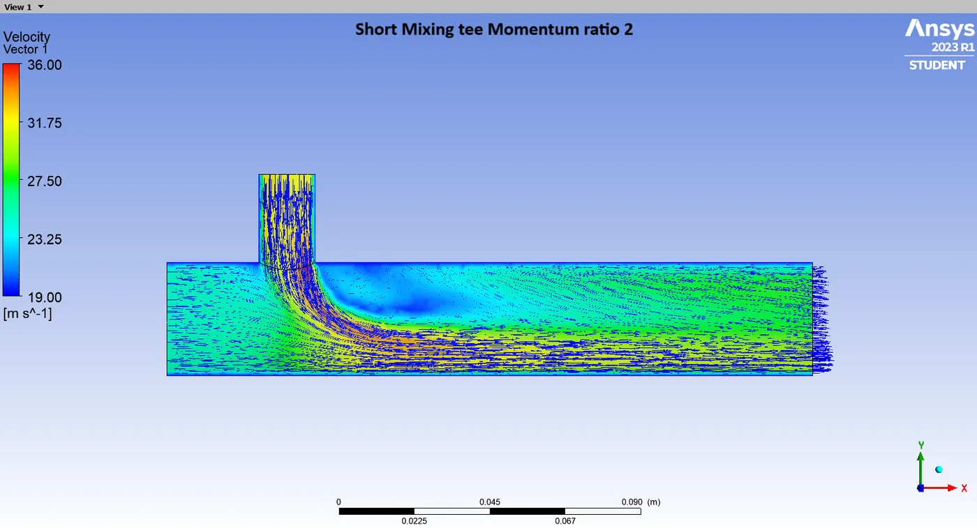
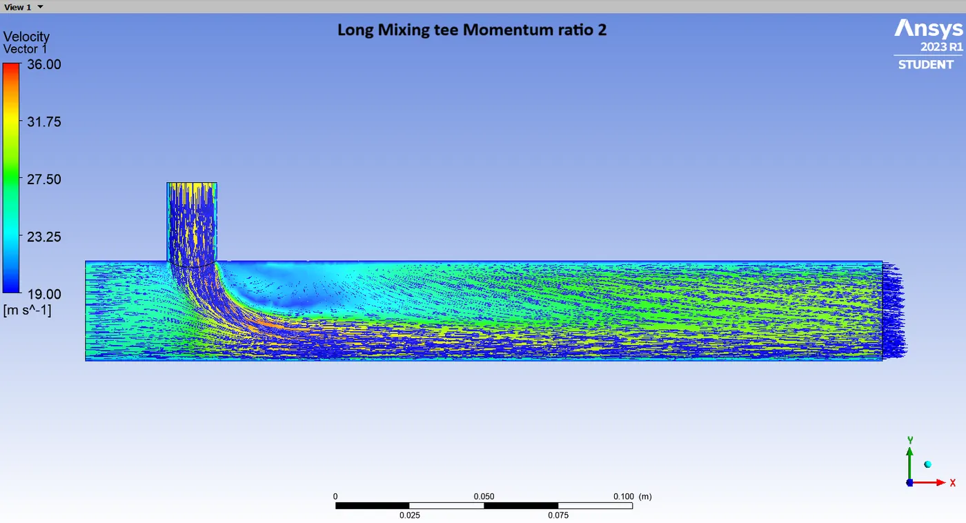
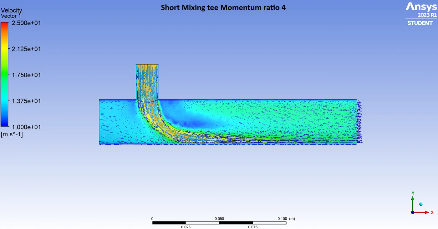
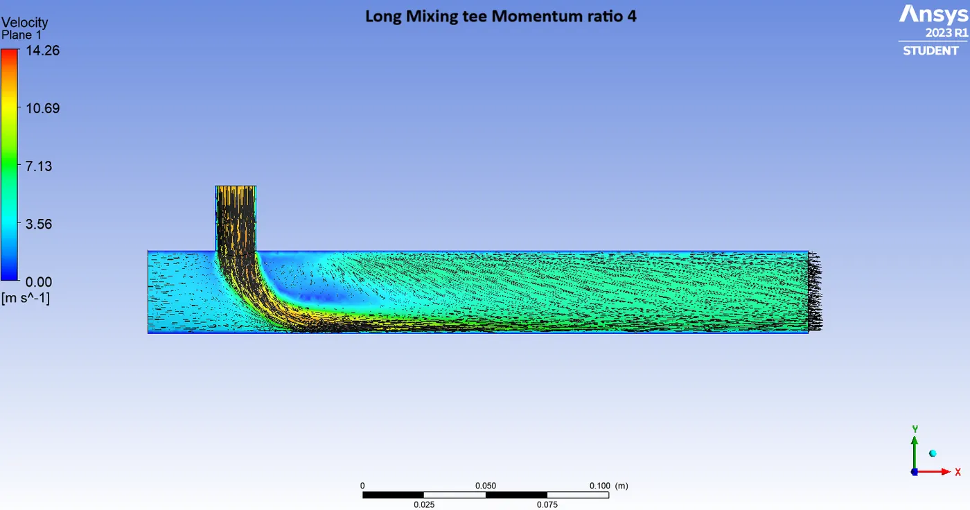
• We also need to find the vector because then only we visualize the fluid flow direction and turbulence flow directions easily. so just select the three arrows icon near the help option. It's called vector 1 After selecting that click OK and Apply.

   

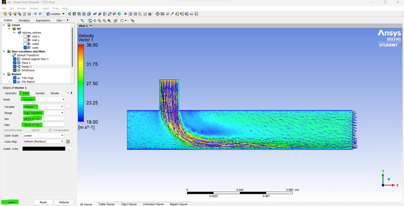
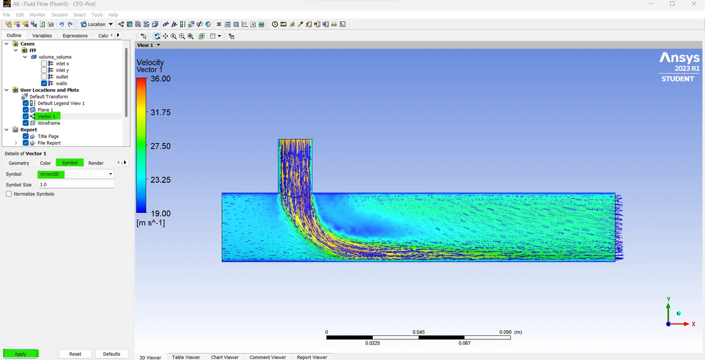
• After applying the vector go to the color section and change the modes into variables. After changing the modes select the variable as a velocity and range as a user specified and we need to give the min value as 19 and maximum as 36 and then just click Apply. And as well as we need to change the symbols like Arrows 3D, 2D, etc.
• Now we can see the vectors along with the velocity result.

RESULT:- 

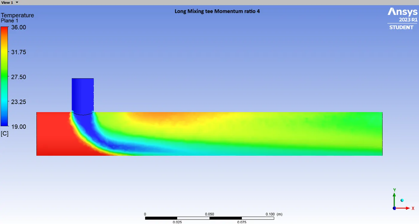
Temperature plot at plane-1 :

 

   

Velocity plot at plain-1 :

 

   

Velocity vector plot at plain-1 :

 

   

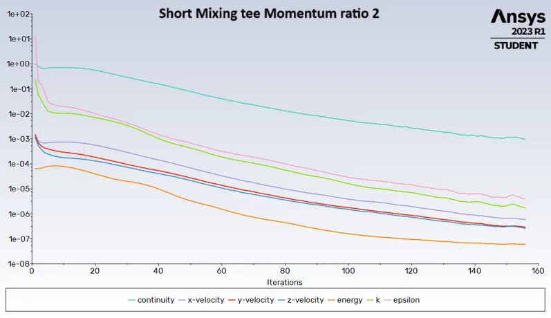
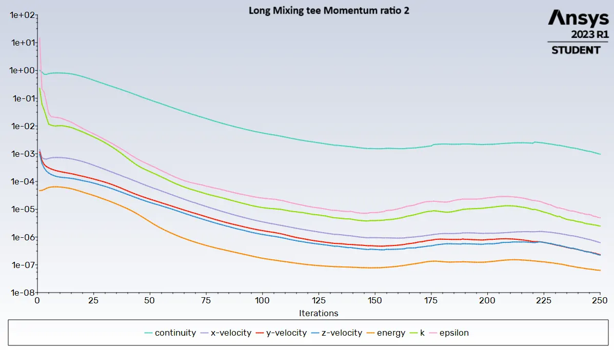
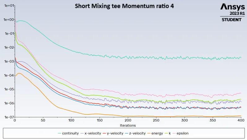
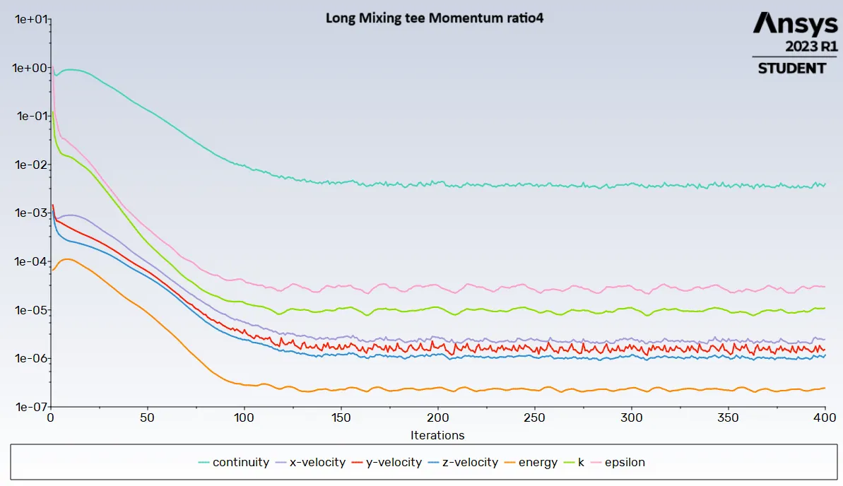
Scaled Residual plots :

   

   

Area weighted Average :

 

   

Standard deviation :

     

 

COMPARISON TABLE:- 

Parameter		Short Tee         MR=2	Short Tee          MR=4	Long Tee               MR=2	Long Tee              MR=4
Cell Count		106249	106249	141303	141303
Temperature           (outlet)°C	Numeric (output) Analytical (output) %Error rate.	30.294367 34.102 5.92%	27.575029 31.875 7.233%	30.406836 34.102 5.73%	27.498448 31.875 7.372%
Velocity             (outlet) m/sec	Numeric (output) Analytical (output) %Error rate.	4.5040935 4.5044 0.0035%	6.0340159 6.0088 0.216%	4.4996505 4.5044 0.054%	6.0176512 6.0088 0.074%
No.of.iterations for convergence.		156	400	250	400

CONCLUSION:-

From this analysis of the above result, it can be concluded that.

1. To get good mixing we see that the velocity of the chilled air is very important. By increasing the velocity of chilled air by a factor of 2 we can able to reduce the outlet temperature quite nicely.
2. The longer pipe configuration is not at all helpful because mostly it gives very similar results to our baseline configurations. when we increase the velocity we will get better turbulent mixing.
3. So, according to the momentum ratios 2 and 4. the MR4 gives better turbulent mixing so that the outlet temperature has been reduced nicely compared with MR2. 
4. Finally the short mixing tee and long mixing tee at momentum ratio 4 give better mixing efficiency and outlet temperature and also give less error rate.