Week 1- Mixing Tee

Aim:

• Set up steady-state simulations to compare the mixing effectiveness when the hot inlet temperature is 36⁰C & the Cold inlet is at 19⁰C
• Understand the difference between the k-epsilon and k-omega SST model for the first case
• Simulate each case for the given velocity and momentum ratio
• Compare results from the 2 cases about cell count, average outlet temperature, and the number of iterations for convergence
• Velocity and temperature contour plots on the cut planes along and across the pipe
• Velocity and temperature line plots along and across the length of the pipe
• Perform Mesh independent study for any one case
• Discuss the effect of length and momentum ratio on the results

Problem Setup:

Case-1

Short mixing tee

a. Simulation-1

Hot Inlet velocity - 3 m/s

Momentum ratio - 4

Cold Inlet velocity - 12 m/s

b. Simulation-2

hot Inlet velocity - 3 m/s

Momentum ratio - 2

Cold Inlet velocity - 6 m/s

Case-2

Long mixing tee

a. Simulation-3

Hot Inlet velocity - 3 m/s

Momentum ratio - 4

Cold Inlet velocity - 12 m/s

b. Simulation-4

Hot Inlet velocity - 3 m/s

Momentum ratio - 2

Cold Inlet velocity - 6 m/s

Let's start with simulation-1 to compare the k-epsilon and k-omega SST models.

Drag and drop the mesh setup to load the geometry and mesh it.

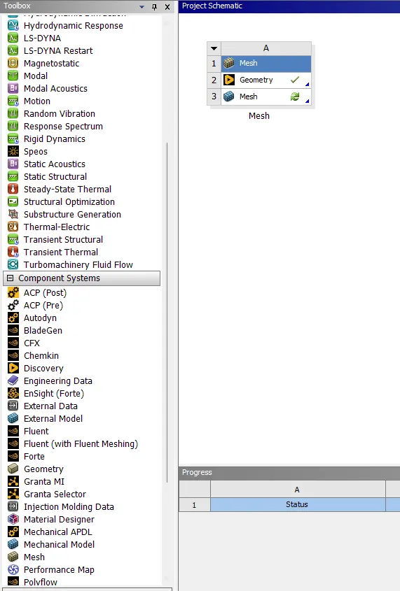
Once the geometry is loaded in the Discovery, use the Volume Extract option to extract the required volume for simulation.

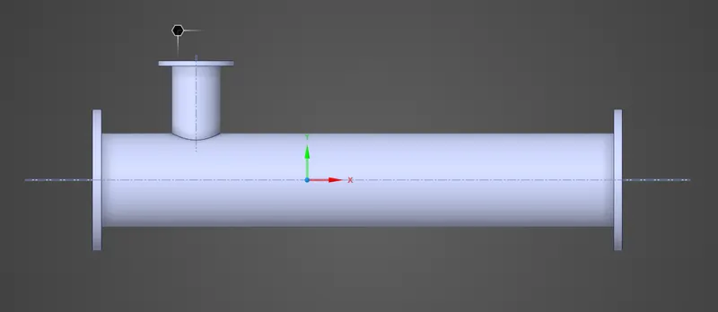
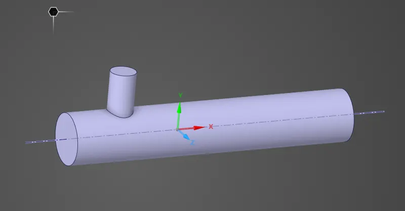
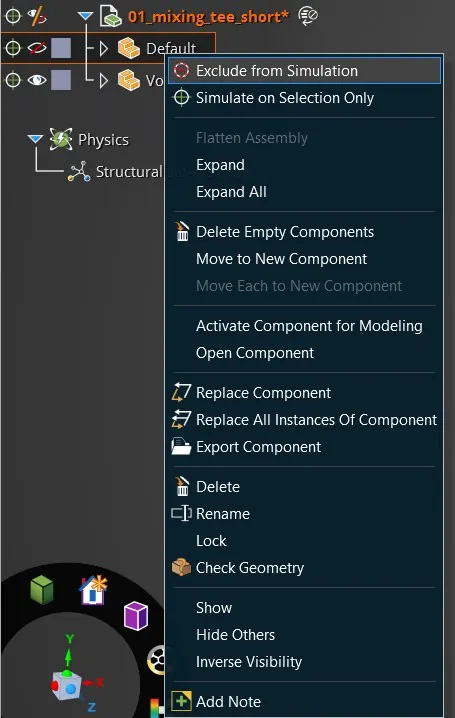
Right-click on Default and click on Exclude from simulation.

Now, proceed to mesh.

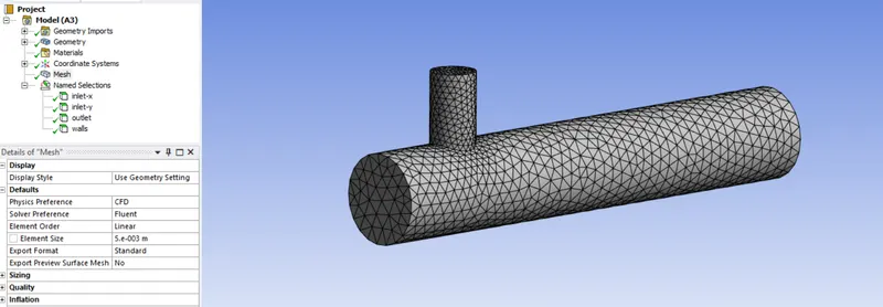
After meshing, start Fluent.

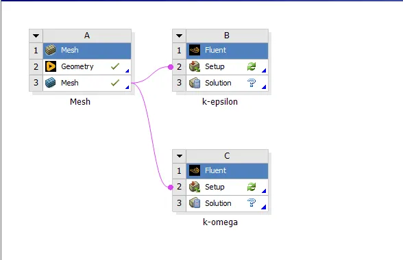
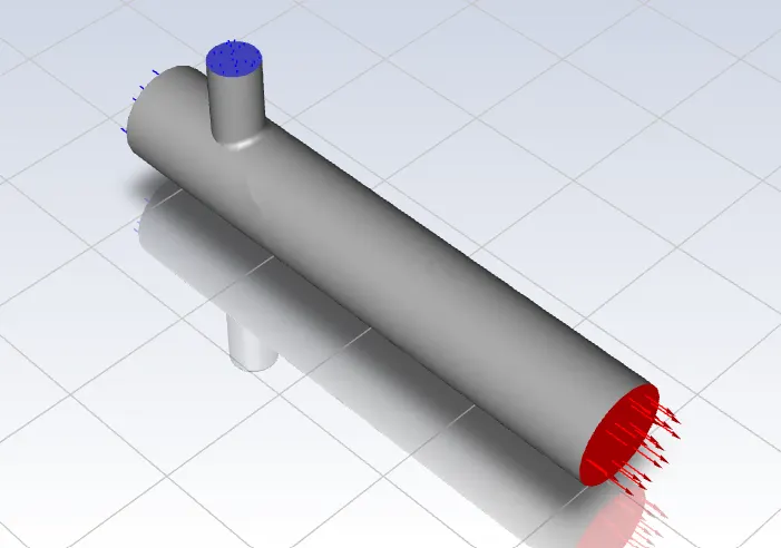
Always remember to perform a mesh check.

Next, go to physics and activate models. First, Turn on the Energy equation. Activating the energy equation allows the temperature-dependent problem to be solved.

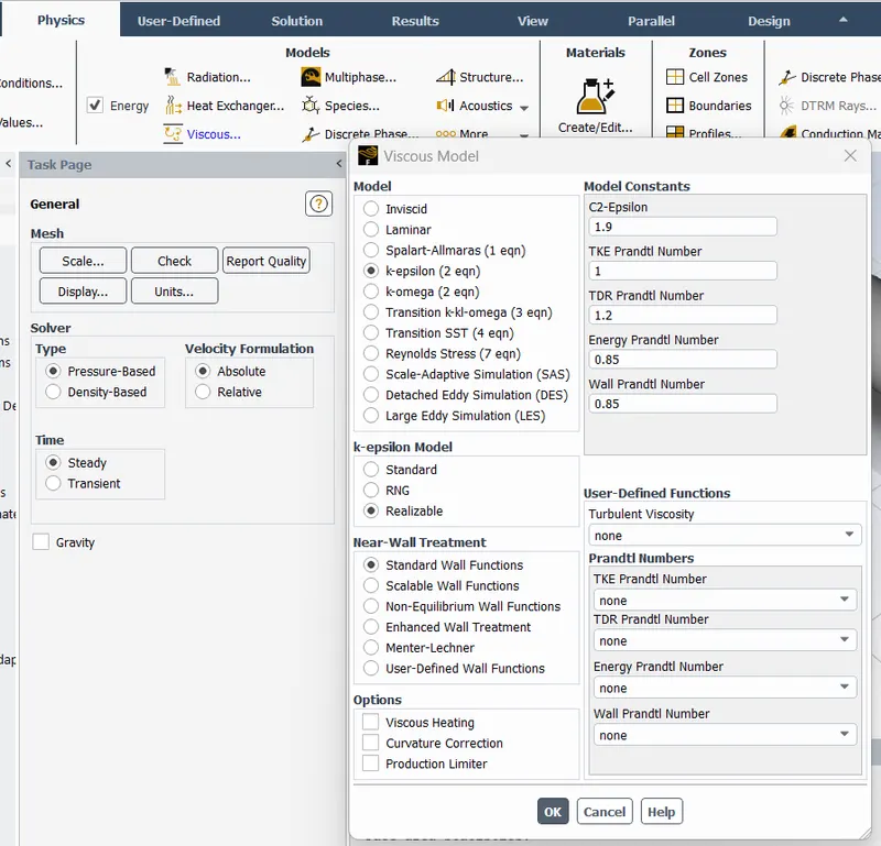
Then, click on the Viscous model and select k-epsilon and Realizable on the k-epsilon model. Leave other settings to be default.

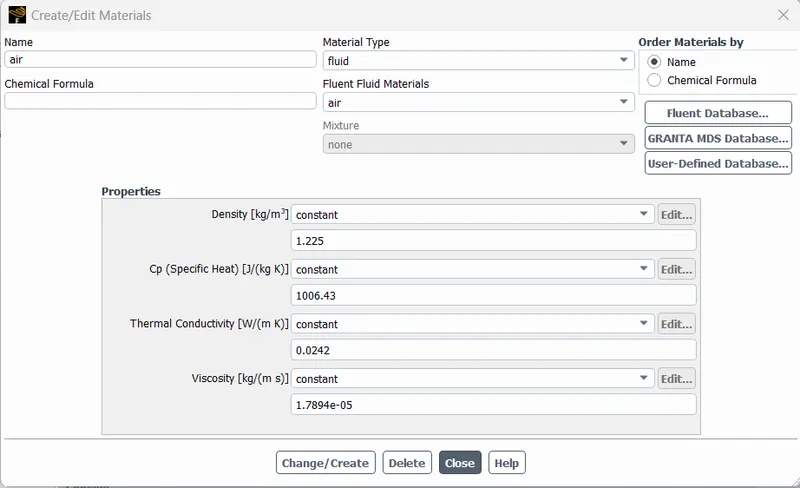
In materials, click on Fluent Database to add new materials. In our case, air is the working fluid.

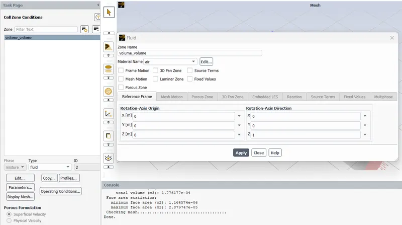
In the cell zone, make sure the working fluid is correct.

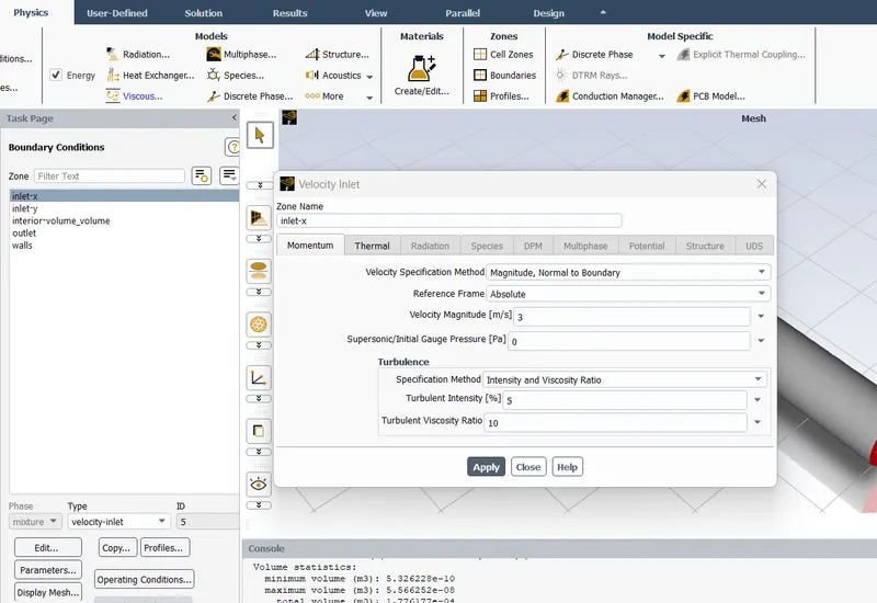
In the Boundary conditions, click on the inlet-x and edit the inlet parameters. Set Velocity mag as 3 m/s and in thermal, set temperature as 36 deg C.

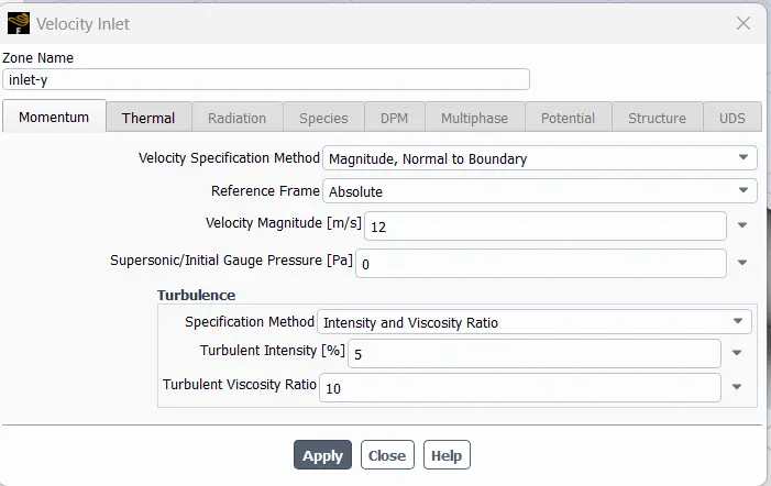
Similarly, for inlet-y set velocity as 12 m/s and temp as 19 deg C.

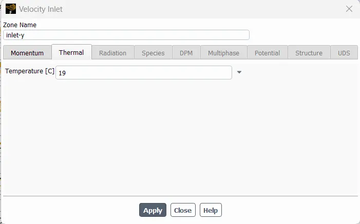
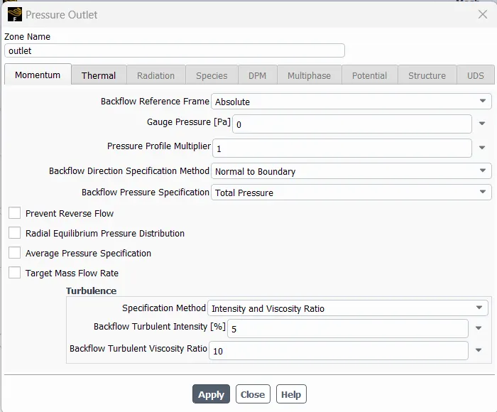
For the outlet, we need atmospheric pressure, and here it is automatically set as gauge pressure to zero which is the same.

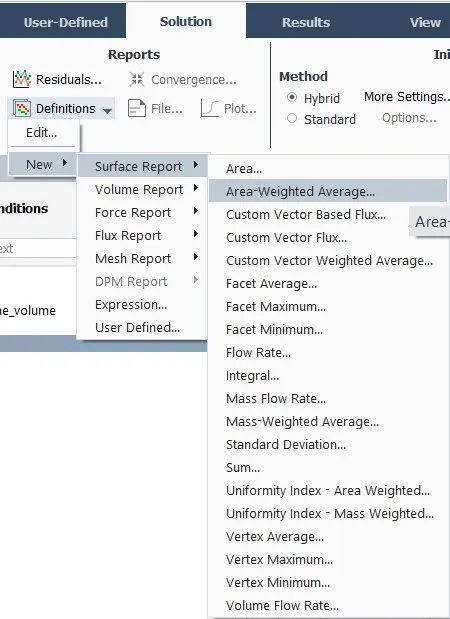
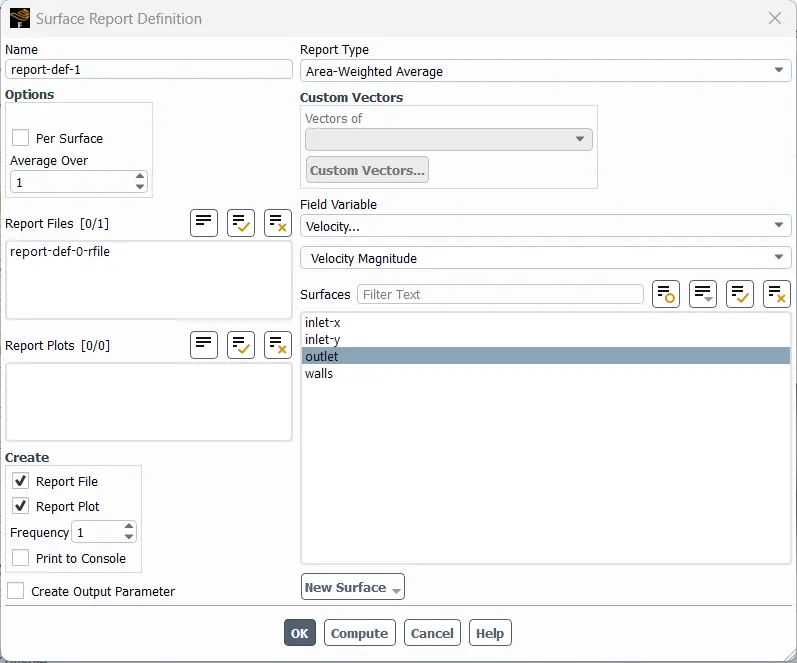
Now, move to Solutions. Click on Definitions>New>Surface Report>Area weighted avg

Here, our requirement is the average temperature at the outlet. Select temperature and outlet.

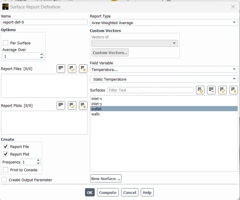
Similarly, create another report for the velocity at the outlet.

Next, click on hybrid initialization.

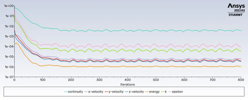
Once, the initialization is complete, set the no. of iterations and click on Calculate.

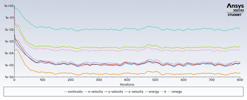
Convergence plot:

Now, proceed to the results.

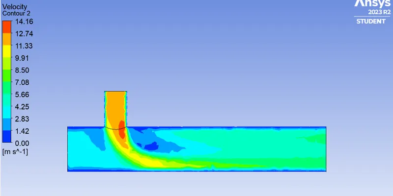
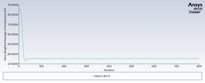
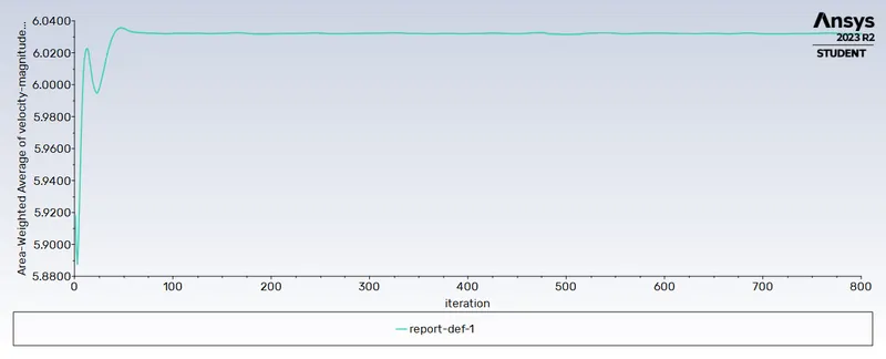
k-omega SST method:

Plots:

Post-processing:

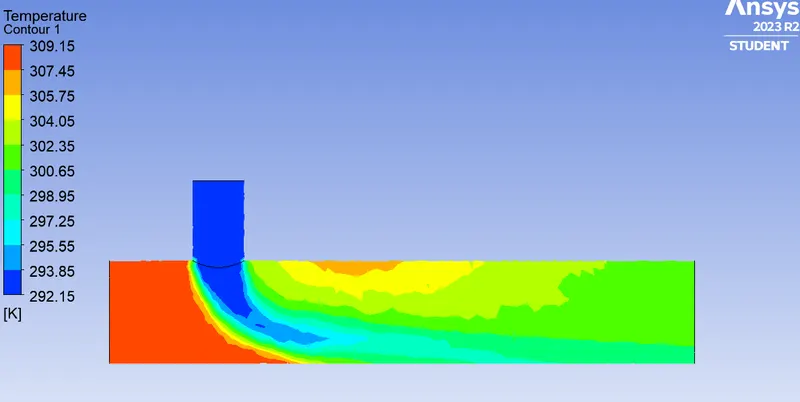
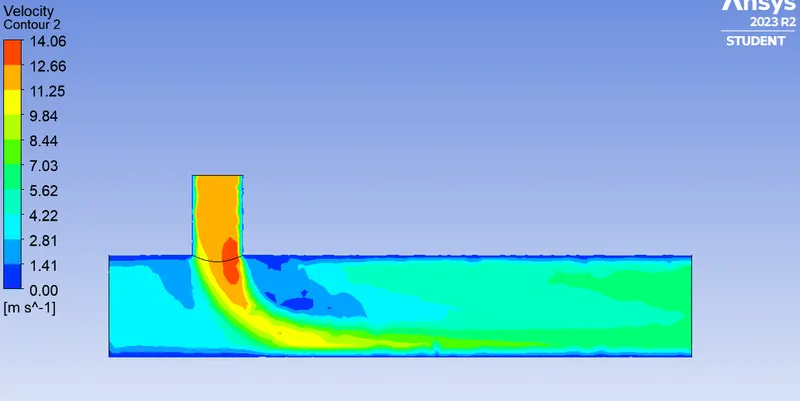
Difference:

The k- omega model is well suited for simulating flow in the viscous sub-layer (near the boundary). On the contrary, The k-epsilon model is ideal for predicting flow in the regions away from the wall.

In our case, we are not working with the walls so we will proceed with the k-epsilon method.

Case 1:

Short mixing tee

a. Simulation-1

Hot Inlet velocity - 3 m/s

Momentum ratio - 4

Cold Inlet velocity - 12 m/s

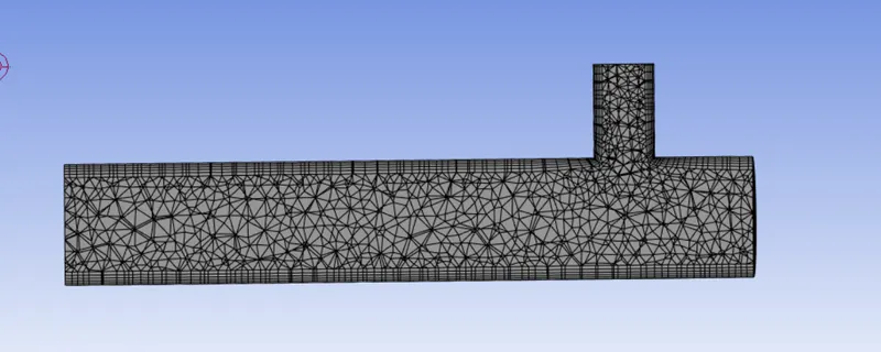
Mesh with inflation:

Results:

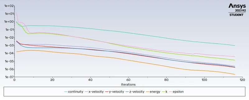
The solution converged at 116 iterations.

Plots:

Residue plot:

Temperature:

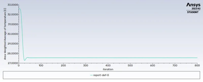
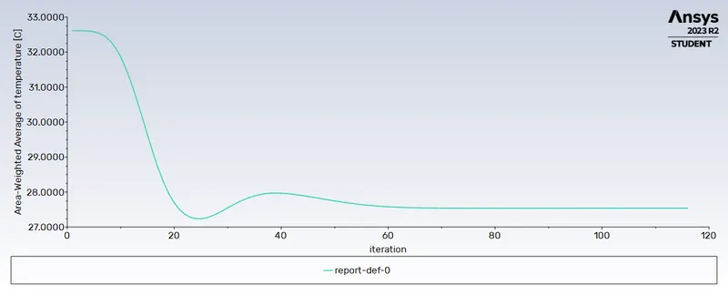
Area weighted average outlet temperature:

The average temperature at the outlet is 27.5373^oC

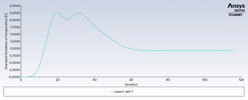
Standard deviation:

The std dev of temperature is around 0.9276. The mixing is good as the std dev is less than 1.

Velocity:

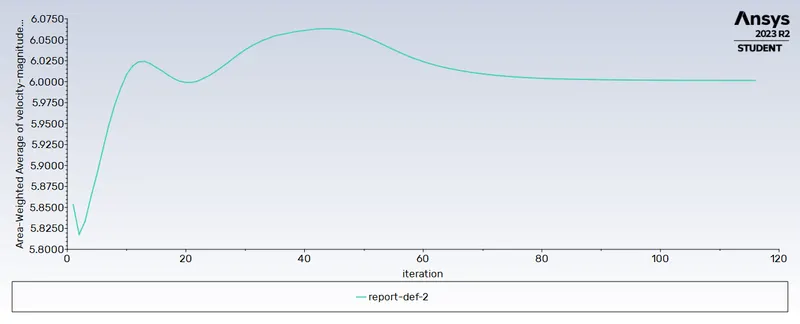
Area-weighted average of velocity magnitude at outlet:

The average velocity at the outlet is 6.0014 m/s.

Post-processing Results:

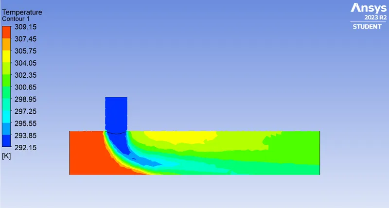
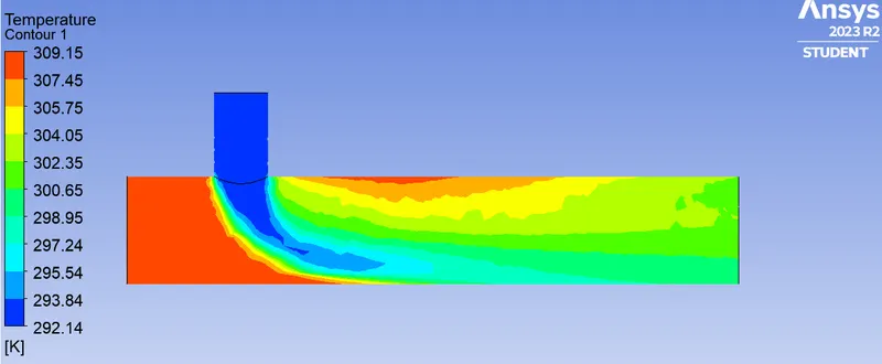
Contour plot:

Temperature:

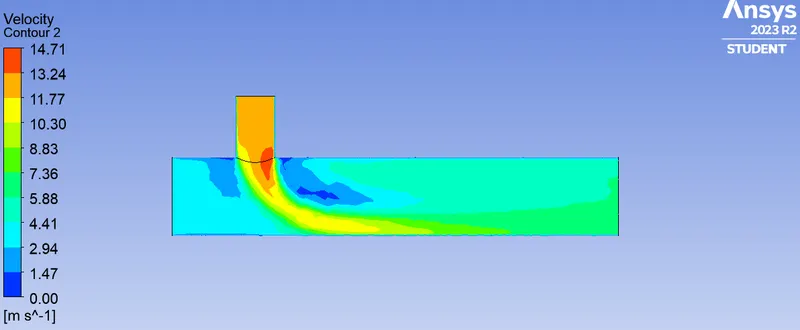
Velocity:

Line plot:

b. Simulation-2

Hot Inlet velocity - 3 m/s

Momentum ratio - 2

Cold Inlet velocity - 6 m/s

Results:

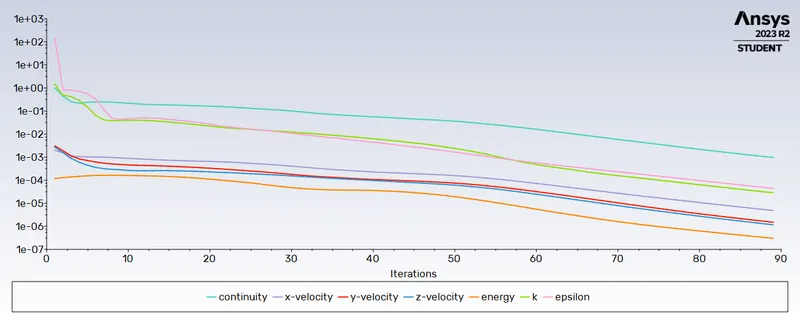
The solution converged at 89 iterations.

Plots:

Residue plot:

Temperature:

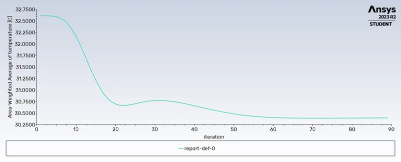
Area weighted average outlet temperature:

The average temperature at the outlet is 30.3976^oC

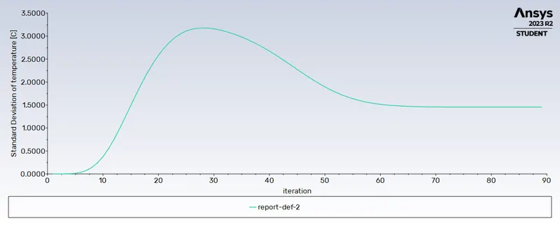
Standard deviation:

The std dev of temperature is around 1.4557. The value is quite large which means the mixing is poor. This is due to the low velocity of the cold inlet.

Velocity:

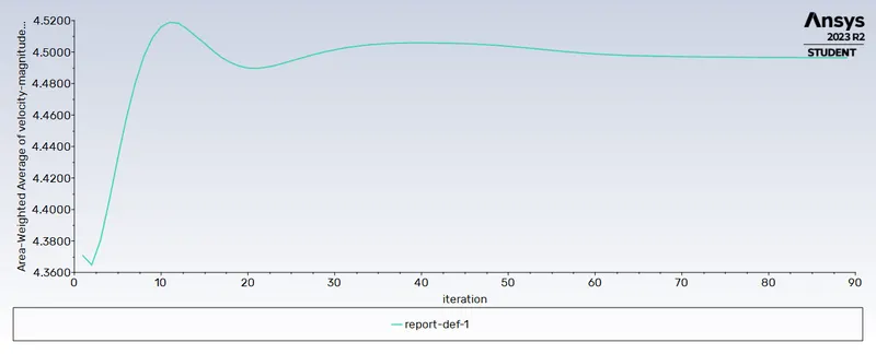
Area-weighted average of velocity magnitude at outlet:

The average velocity at the outlet is 4.4964 m/s.

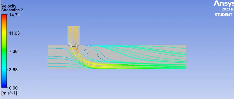
Post-processing Results:

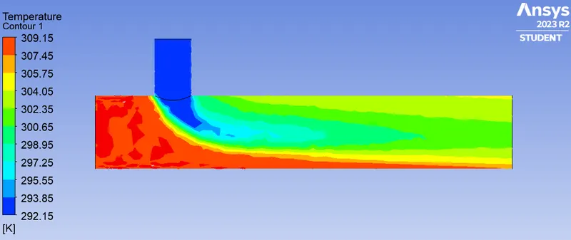
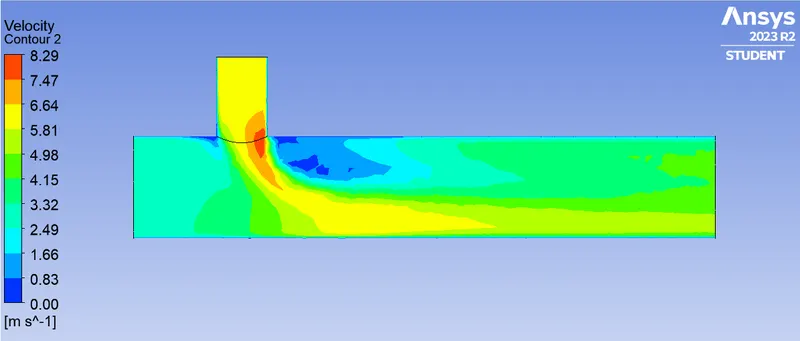
Contour plot:

Temperature:

Velocity:

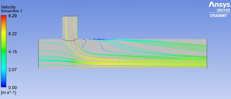
Line plot:

Case-2

Long mixing tee

a. Simulation-3

Hot Inlet velocity - 3 m/s

Momentum ratio - 4

Cold Inlet velocity - 12 m/s

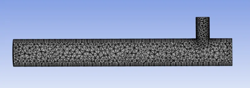
Mesh with inflation:

Results:

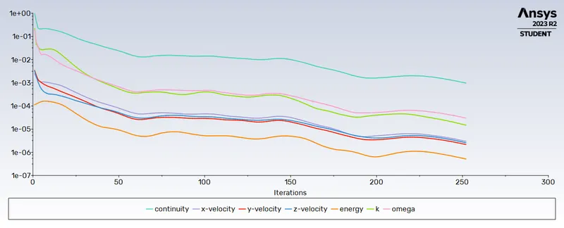
The solution converged at 252 iterations.

Plots:

Residue plot:

Temperature:

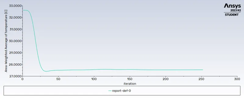
Area weighted average outlet temperature:

The average temperature at the outlet is 27.5461^oC

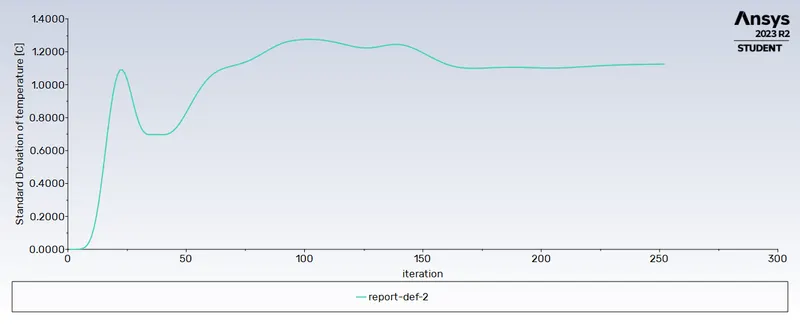
Standard deviation:

The std dev of temperature is around 1.1253. The mixing is fair as the std dev is closer to 1.

Velocity:

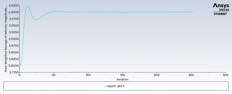
Area-weighted average of velocity magnitude at outlet:

The average velocity at the outlet is 6.0002 m/s.

Post-processing Results:

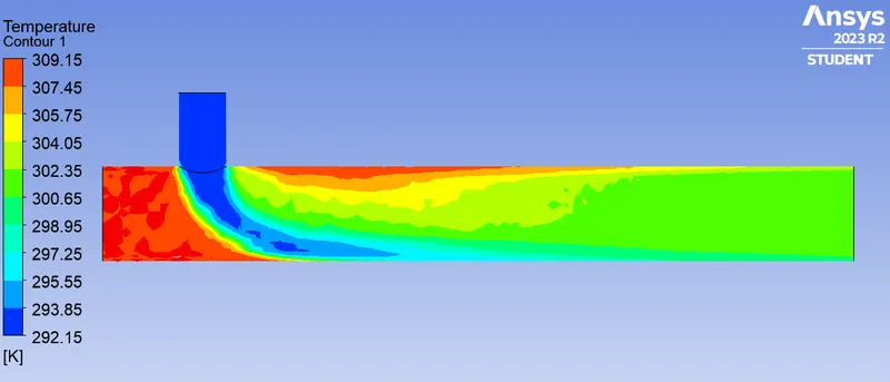
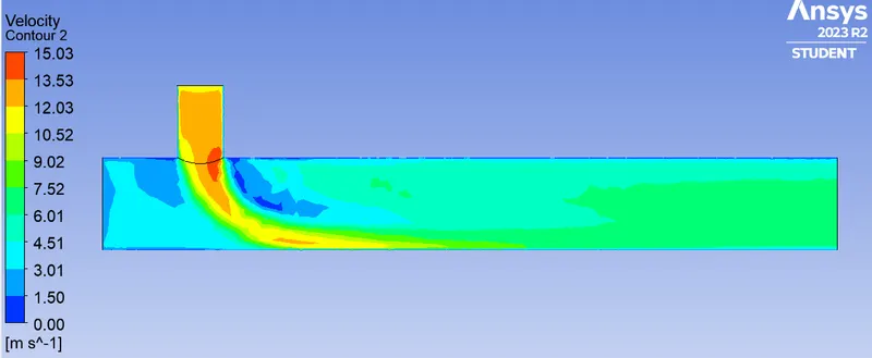
Contour plot:

Temperature:

Velocity:

Line plot:

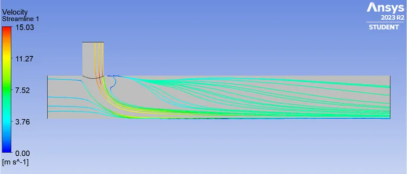
b. Simulation-4

Hot Inlet velocity - 3 m/s

Momentum ratio - 2

Cold Inlet velocity - 6 m/s

Results:

The solution converged at 96 iterations.

Plots:

Residue plot:

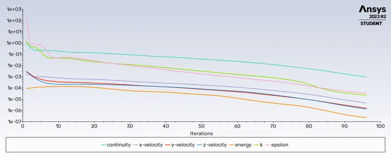
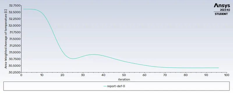
Temperature:

Area weighted average outlet temperature:

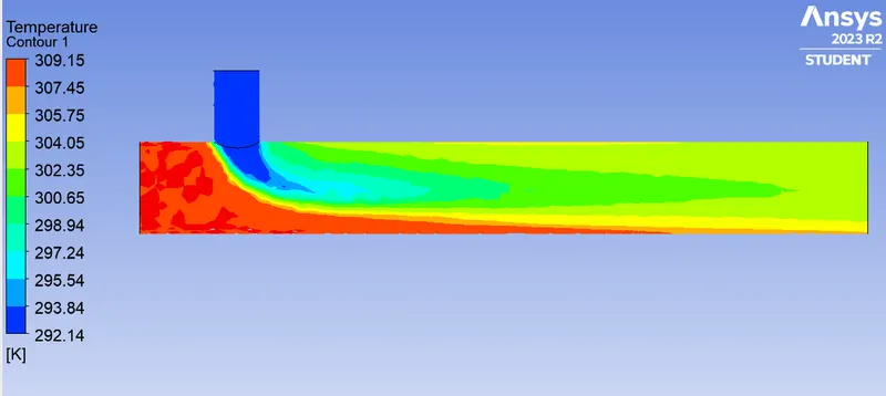
The average temperature at the outlet is 30.4191^oC

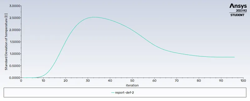
Standard deviation:

The std dev of temperature is around 0.8598. The mixing is good as the std dev is less than 1.

Velocity:

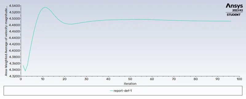
Area-weighted average of velocity magnitude at outlet:

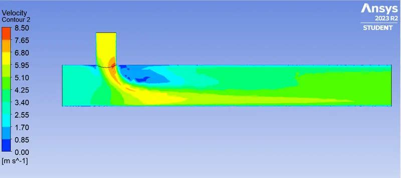
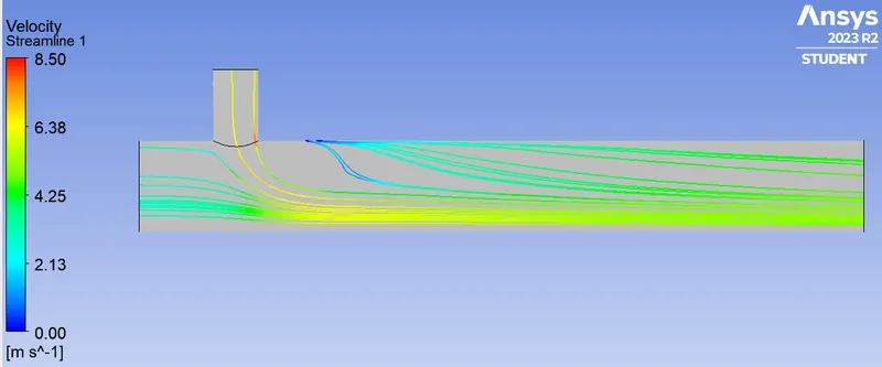
The average velocity at the outlet is 4.4918 m/s.

Post-processing Results:

Contour plot:

Temperature:

Velocity:

Line plot:

Mesh independence:

The mesh independence test was done by running 3 simulations on the Short mixing tee case for both momenta.

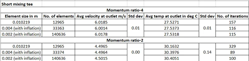
A mesh independence study is done to determine the dependence of the results on the mesh density.

The standard deviation of these values is close to zero. Therefore, it passes the mesh independence test.

Conclusion:

• The k-epsilon models predict flow far from the boundaries, and the k-omega model predicts flow near the boundaries. In our case, the simulation model is a turbulent flow far from the boundaries; therefore, the k-epsilon model is used.
• The mixing of fluids was better at the high velocity of inlet flow. A higher momentum ratio gives rise to better mixing of fluids at the outlet.
• As the length of the pipe was increasing, the mixing was better due to the diffusion.
• Therefore, a long mixing tee with increased momentum is better considering diffusion. If diffusion is not considered, then the short mixing tee with momentum is sufficient.