Week 2 Air standard Cycle
Objectives:
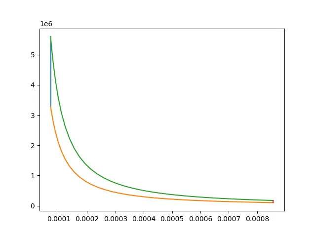
To solve the otto cycle and plot the PV diagram and also calculate the thermal efficiency of the engine.
Parameters:
Inlet Pressure, p1=101325 Pa
Initial Temperature, t1=500 K
gamma=1.4
Geometric parameters:
bore=0.1 m
stroke=0.1 m
Connecting rod length, con_rod=0.15 m
Compression ratio, cr=12
Temperature, t3 = 2300 K (Assumed)
Solution:
- The required libraries are imported
- The function engine_kinematics was defined which calculates the volume
- Outside the function block, the given parameters and the formulas to calculate the required values were coded
- The function call was initiated for compression as well as expansion cycles with varying TDC and BDC
- Then the thermal efficiency was calculated
- At last, the PV diagram was plotted using matplotlib library
Results:
- The PV diagram is plotted
- The Thermal Efficiency is= 62.9892%
import math
import matplotlib.pyplot as plt

def engine_kinematics(bore,stroke,con_rod,cr,start_crank,end_crank):
    a=stroke/2
    R=con_rod/a

    #Volume
    V_s=math.pi*(1/4)*pow(bore,2)*stroke
    V_c=V_s/(cr-1)

    #crank angle
    theta=math.radians(180)

    sc=math.radians(start_crank)
    ec=math.radians(end_crank)

    num_values=50
    dtheta=(ec-sc)/(num_values-1)
    v=[]
    for i in range(0,num_values):
        theta=sc+i*dtheta
        term1=0.5*(cr-1)   #V/Vc eqn split into 3 terms
        term2=R+1-math.cos(theta)
        term3=pow(R,2)-pow(math.sin(theta),2)
        term3=pow(term3,0.5)
        v.append((1+term1*(term2-term3))*V_c)
    return v


#inputs-state point-1
p1=101325
t1=500
gamma=1.4

#geometric parameters
bore=0.1
stroke=0.1
con_rod=0.15
cr=12    #compression ratio

#Volume computation
v_s=(math.pi/4)*pow(bore,2)*stroke  #swept volume
v_c=v_s/(cr-1)  #clearance volume
v1=v_c+v_s

#state point-2
v2=v_c

#p2v2^gamma=p1v1^gamma
p2=p1*pow(v1,gamma)/pow(v2,gamma)   #Isentropic equation

#p2v2/t2=p1v1/t1 | rhs=p1v1/t1 | p2v2/t2=rhs | t2=p2v2/rhs
rhs=p1*v1/t1
t2=p2*v2/rhs

V_compression=engine_kinematics(bore,stroke,con_rod,cr,180,0)
constant=p1*pow(v1,gamma)

P_compression=[]
for v in V_compression:
    P_compression.append(constant/pow(v,gamma))

#state point-3
v3=v2
t3=2300  #assumed temperature

#p3v3/t3=p2v2/t2 |rhs=p2v2/t2|p3=rhs*t3/v3
rhs=p2*v2/t2
p3=rhs*t3/v3

V_expansion=engine_kinematics(bore,stroke,con_rod,cr,0,180)
constant=p3*pow(v3,gamma)

P_expansion=[]
for v in V_expansion:
    P_expansion.append(constant/pow(v,gamma))

#state point-4
v4=v1

#p4v4^gamma=p3v3^gamma
p4=p3*pow(v3,gamma)/pow(v4,gamma)

#p4v4/t4=p4v3/t3=rhs
t4=p4*v4/rhs

#Thermal Efficiency calculation
Efficiency= 1-((t4-t1)/(t3-t2))
print('Thermal Efficiency is=', Efficiency*100)

plt.plot([v2,v3],[p2,p3])
plt.plot(V_compression,P_compression)
plt.plot(V_expansion,P_expansion)
plt.plot([v4,v1],[p4,p1])
plt.show()
PV Plot: