Week 3 - Solving second order ODEs

b=0.05

g=9.81 in m/s2

l=1 in m

m=1 in kg

Simulation is done for 0-20 sec, for angular displacement=0,angular velocity=3 rad/sec at time t=0.

Modifying the eqn,

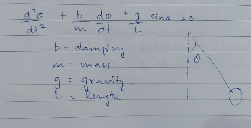
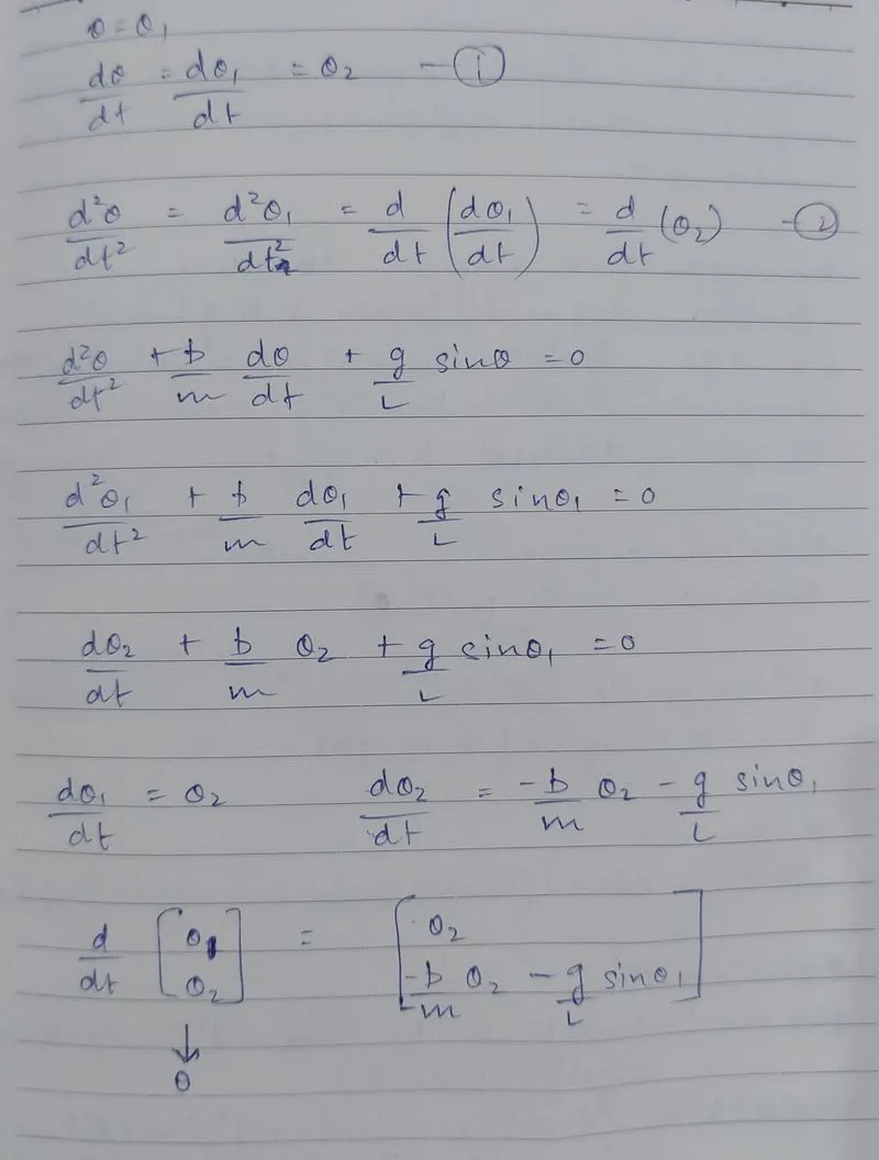
import numpy as np  #for various math functions
from scipy.integrate import odeint  #for solving ode
import matplotlib.pyplot as plt #for plotting data
import math #for using trigonometric functions

#function that returns dtheta/dt

def model(theta,t,b,g,l,m):
    theta1=theta[0]
    theta2=theta[1]
    dtheta1_dt=theta2
    dtheta2_dt=-(b/m)*theta2-(g/l)*math.sin(theta1)  
    dtheta_dt=[dtheta1_dt,dtheta2_dt]
    return dtheta_dt  #returns the value of dtheta_dt to be used outside the function

b=0.05  #b=damping coefficient
g=9.81  #g=gravity in m/s2
l=1     #l=length in m
m=1  #m=mass in kg

#initial conditions
theta_0=[0,3]

#time points
t=np.linspace(0,20,200)

#solve ode
theta=odeint(model,theta_0,t,args=(b,g,l,m))

#plot results
plt.figure()
plt.plot(t,theta[:,0],'b-',label=r'$\frac{d\theta_1}{dt}=\theta2$') #plotting the legend
plt.plot(t,theta[:,1],'r--',label=r'$\frac{d\theta2}{dt}=-\frac{b}{m}\theta_2-\frac{g}{L}sin\theta_1$')  #plotting the legend
plt.ylabel('Plot')  #naming the y-axis 
plt.xlabel('Time')  #naming the x-axis 
plt.legend(loc='best') #automatically chooses the best location for the legend placement
plt.show()


#Animation
ct=1

for i in theta[:,0]:
    x0=0  #initializing x0 coordinate
    y0=0  #initializing y0 coordinate
    x1=l*math.sin(i) #initializing x1 coordinate
    y1=-(l*math.cos(i)) #initializing y1 coordinate

    filename=str(ct)+'.png'  #saving the filename in sequential order
    ct=ct+1 #incrementing ct for the loop

    #plot
    plt.figure()
    plt.plot([-0.5,0.5],[0,0],linewidth=4,color='black') #plotting the base of the pendulum
    plt.plot([x0,x1],[y0,y1],linewidth=2,color='g')  #plotting the string
    plt.plot(x1,y1,'o',markersize=10,color='r')  #plotting the sphere
    plt.xlim([-2,2]) #defining x-axis limits
    plt.ylim([-2,2])  #defining y-axis limits
    plt.title('Animation of Simple Pendulum')
    plt.savefig(filename)

Output:

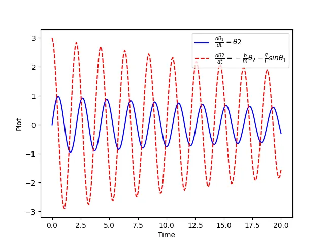
In the plot shown above, the blue solid line is the displacement and the red dashed line is the velocity. The plot shows the damping as both are decreasing.

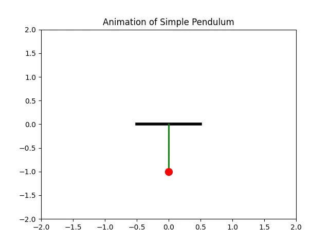
Animation of Simple Pendulum:

Errors Faced during coding:

1. Error due to unrecognized variable 'Loc'. It was corrected by replacing it with the small letter 'l', loc='best'.

2. Error due to inconsistent use of tabs and spaces in indentation. It was solved by correcting the spaces.

Results and Discussion:

200 images have been saved in a separate folder and stitched together and converted into a gif. The animation shows the simple pendulum oscillation according to the given inputs.