Week 1- Mixing Tee
Aim: To create a steady state simulation of two versions of the mixing tee. One of them is longer than the other, using Ansys Fluent.
Objective:
- Case 1
- Short mixing tee with a hot inlet velocity of 3m/s.
- Momentum ratio of 2, 4.
- Case 2
- Long mixing tee with a hot inlet velocity of 3m/s.
- Momentum ratio of 2, 4.
- To use the k-epsilon and k-omega SST model for the first case.
- To compare a cell count of both cases.
- To compare an average outlet temperature of both cases.
- To compare a number of iterations for convergence.
Given Input
- Hot inlet temperature is 360C.
- Cold inlet is at 190C.
- To use the k-epsilon and k-omega SST model for the first case.
- Momentum ratio = velocity at cold inlet / velocity at hot inlet.
- A hot inlet velocity of 3m/s.
- Momentum ratio of 2, 4.
Theory
- Mixing tee is a type of mixing mechanism. Mixing Tees utilizes a specifically engineered internal geometry to efficiently mix two fluid streams into one combined stream. Mixing tees are widely used in the petrochemical, HVAC industry etc.
- Mixing tee refers to a plumbing fitting that is used to combine or redirect the flow of fluids, typically in pipes or tubing. It is called a "tee" because it has a shape that resembles the letter "T", with two inlets and one outlet at right angles to each other.
- Mixing tees are commonly used in plumbing systems to blend different fluids or substances together, such as hot and cold water in a plumbing system for controlling the temperature of the water being delivered to a faucet or a shower. They are also used in industrial processes, chemical processing plants, and other applications where it is necessary to combine or redirect the flow of fluids.
- Mixing tees can be made of various materials, such as brass, copper, stainless steel, PVC, or other materials depending on the specific application and the type of fluids being mixed. They typically have threaded, soldered, or glued connections for easy installation into a plumbing or piping system.
- It's important to note that the specific design and functionality of a mixing tee may vary depending on the application and requirements. For complex or specialized applications, it's always best to consult with a qualified plumber or engineer to ensure proper selection and installation of mixing tees for optimal performance and safety.
- Application of mixing tee.
- Plumbing systems
- HVAC systems
- Industrial processes
- Water treatment systems
- Agriculture and irrigation systems
- Process control systems
- Renewable energy systems
Images of model
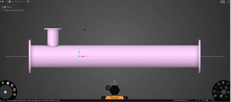
- Long mixing tee
Procedure
- Step 1:- Geometry
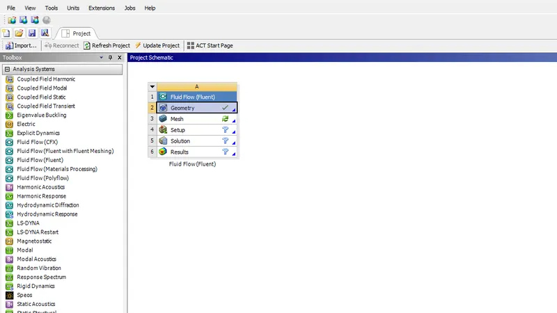
- Inserting a Fluid Flow (Fluent) and, Importing the geometry in the workbench.
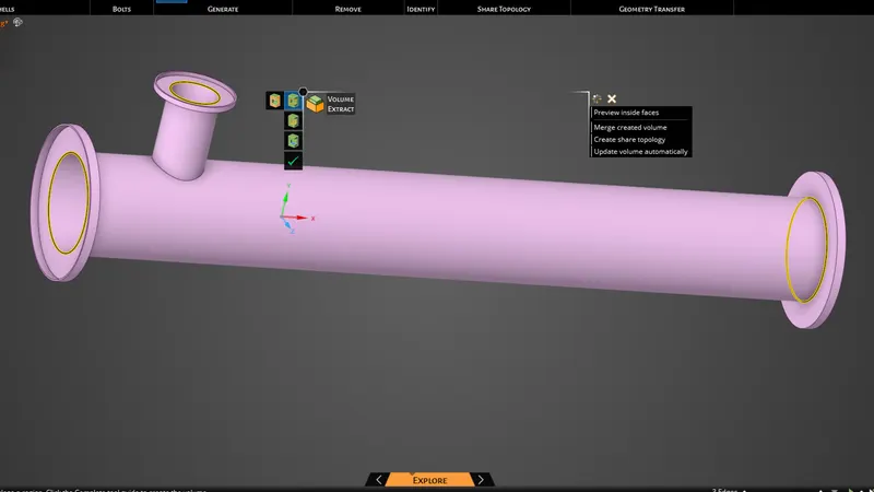
- Prepare> Volume Extract> Edge> Select all the three edges of the mixing tee.
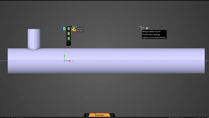
- Included in simulation is used for hiding an edge which are selected. Now close the file, it will save automatically.
- Inserting a Fluid Flow (Fluent) and, Importing the geometry in the workbench.
- Step 2:- Mesh
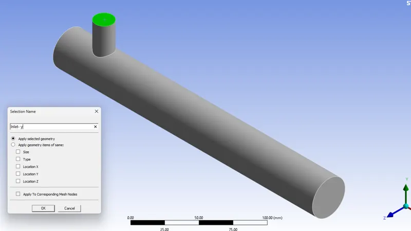
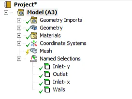
- Give Labeling to the surface.
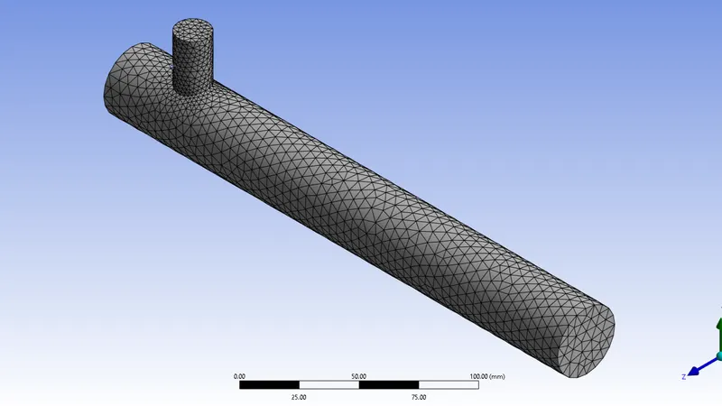
- Mesh Generation for the model.
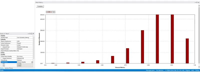
- Mesh Metric> Element Quality
- Section Plane is use to cut the model into to parts, It is use for seeing the genertared mesh in inside volume.
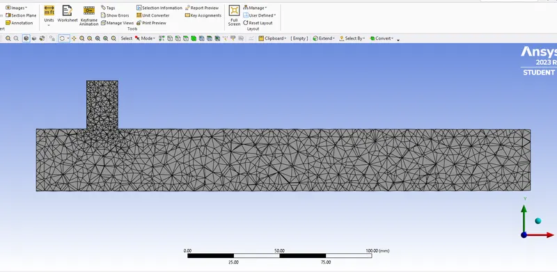
- Give Labeling to the surface.
- Case 1
- Step 3:- Setup
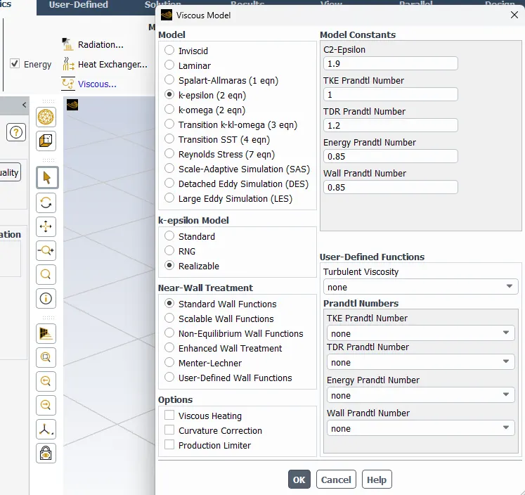
k-epsilon hot inlet velocity of 3m/s.
- Mesh checkup
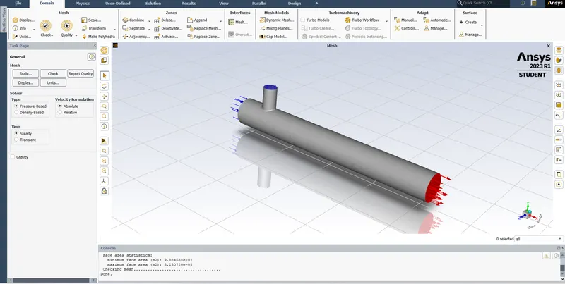
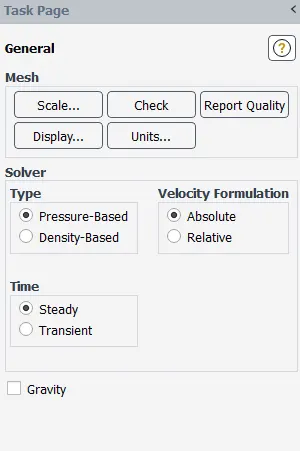
- Coundistions
- K- Epsilon
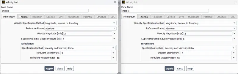
- Boundary condition of Inlet-x and Inlet-y value
- Definitions for different remote condition
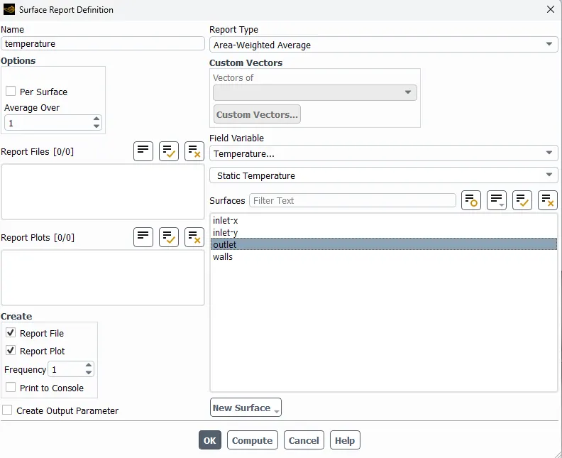
- Temperature
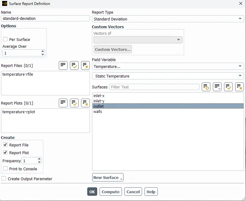
- Standard Deviation
- Temperature
-
Initialize using the hybrid initialization method
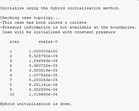
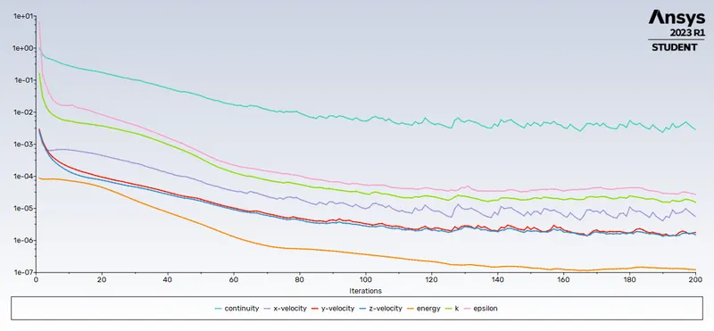
- Scales Residuals
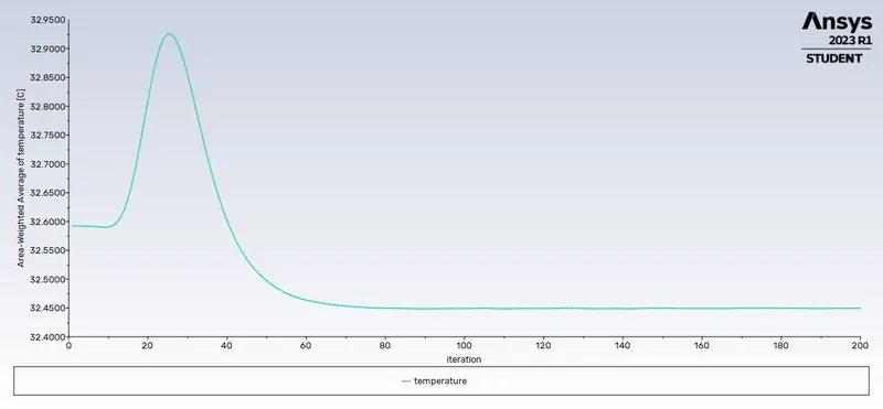
- Temperature
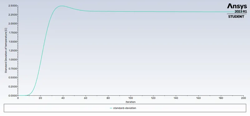
- Standard Deviation
- Mesh checkup
- Step 4:-
- Temperature plane
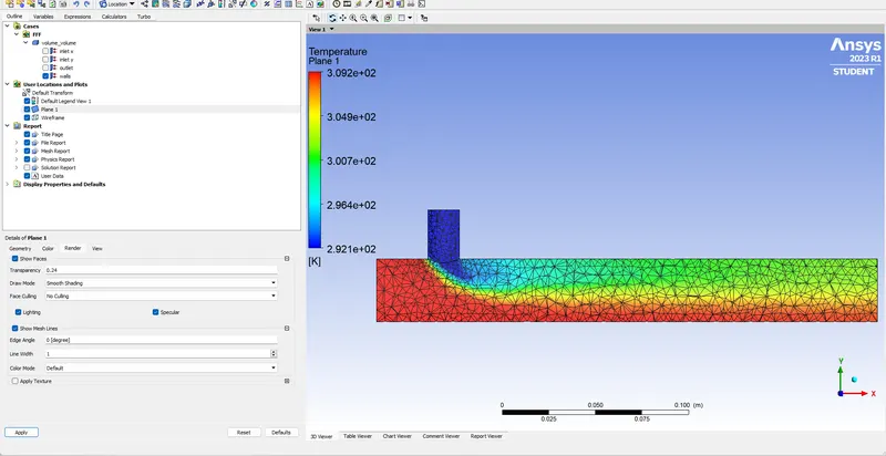
- Temperature in circular plane
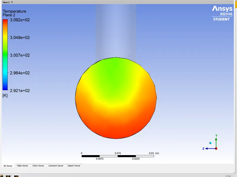
- Temperature plane
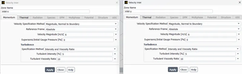
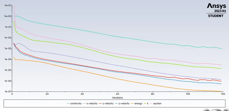
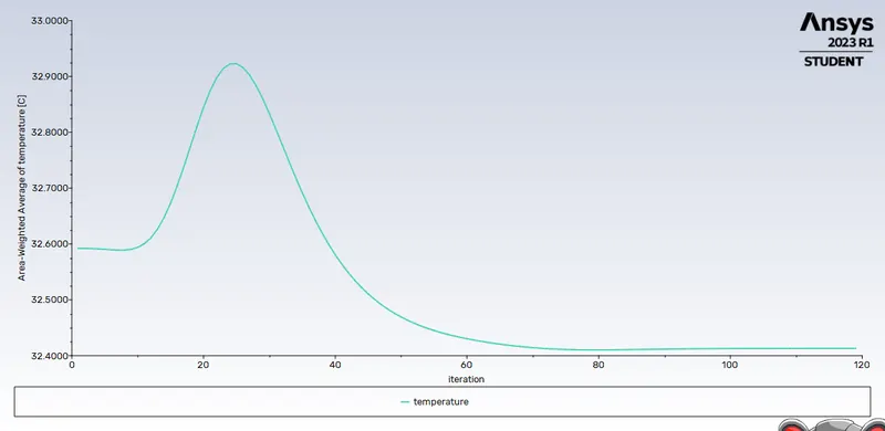
- Post Processed result of K-Epsilon hot inlet velocity of 6m/s. The momentum ratio of 2.
- Boundary condition for Input-x and Input-y.
- Scaled Residuals
- Temperature
- Standard Deviation
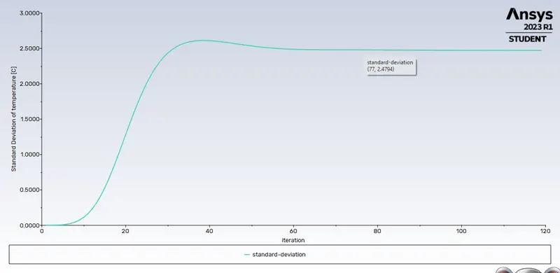
- Compute Calculation
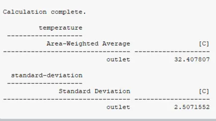
- Boundary condition for Input-x and Input-y.
- Postprocesser Result
- Temperature Plane
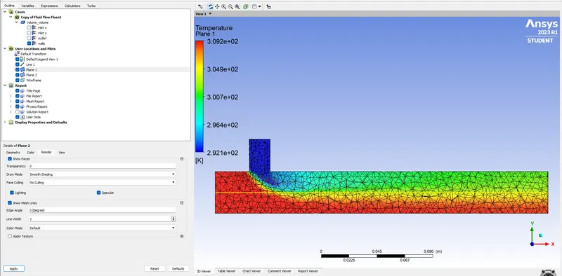
- Circular Plane
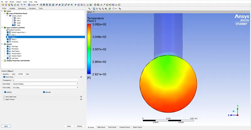
- Chart
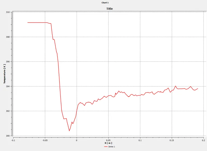
- Temperature Plane
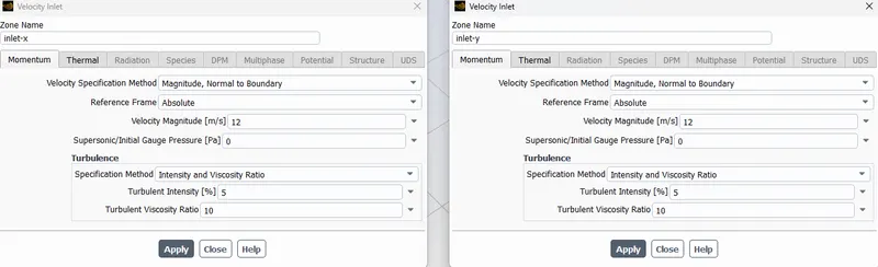
- Post Processed result of K-Epsilon hot inlet velocity of 12m/s. The momentum ratio of 4.
- Boundary conditio for Input-x and Input-y.
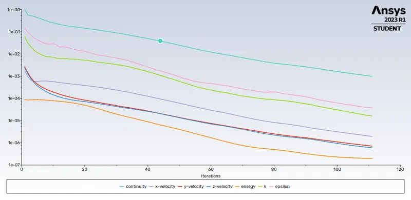
- Scaled Residuals
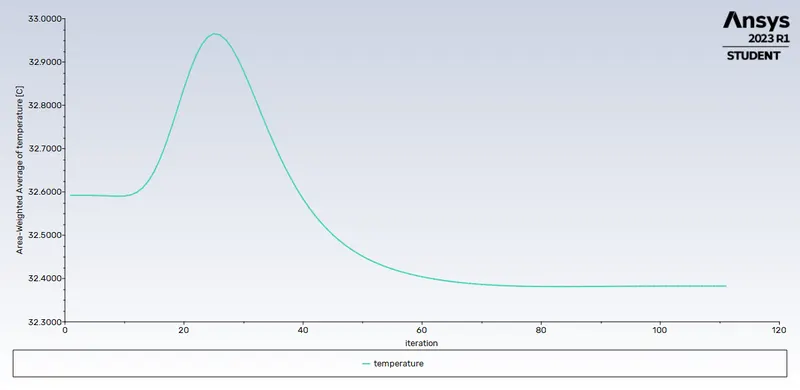
- Temperature
- Standard Deviation
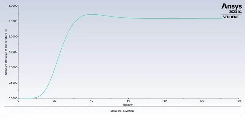
- Compute calculation
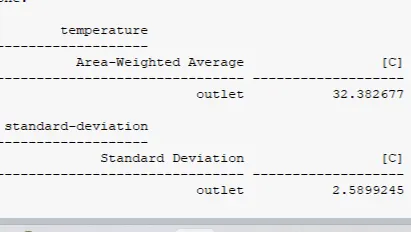
- Boundary conditio for Input-x and Input-y.
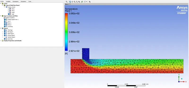
- Postprocesser Result for 12m/sec
- Temperature Plane
- Circular Plan
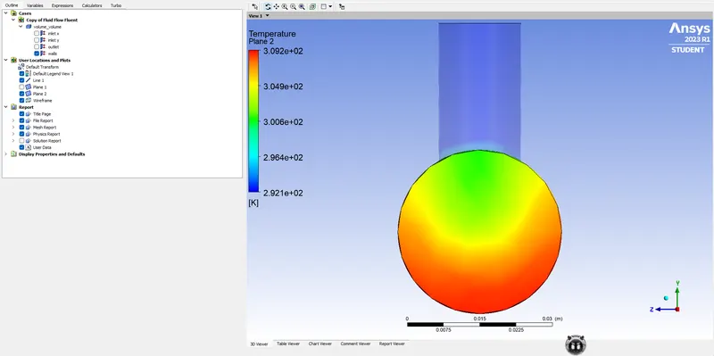
- Chart
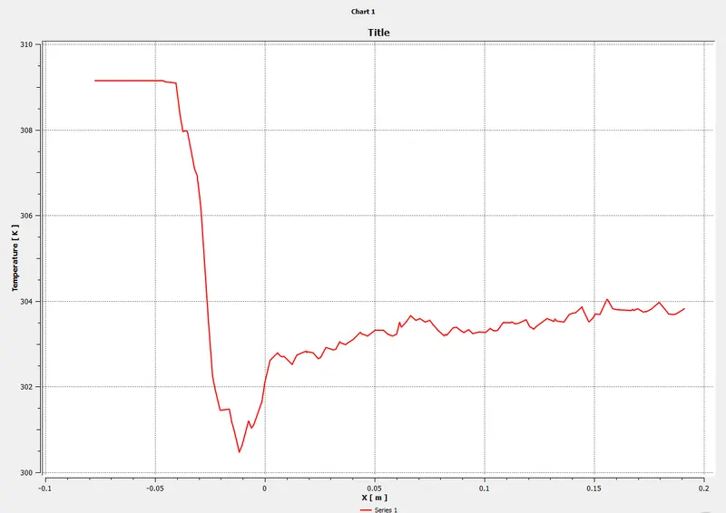
- Temperature Plane
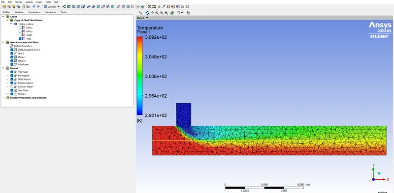
- Post Processed result of K-Omega hot inlet velocity of 3m/s.
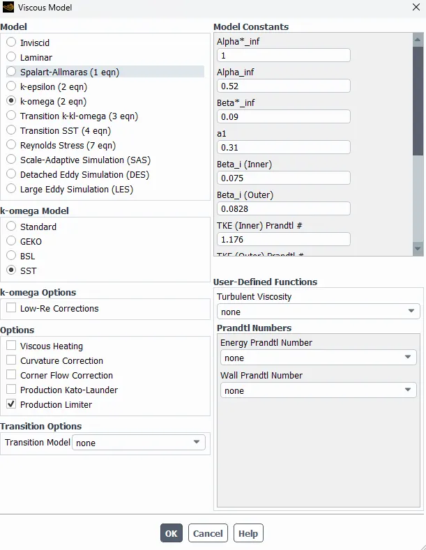
- Boundary Condition
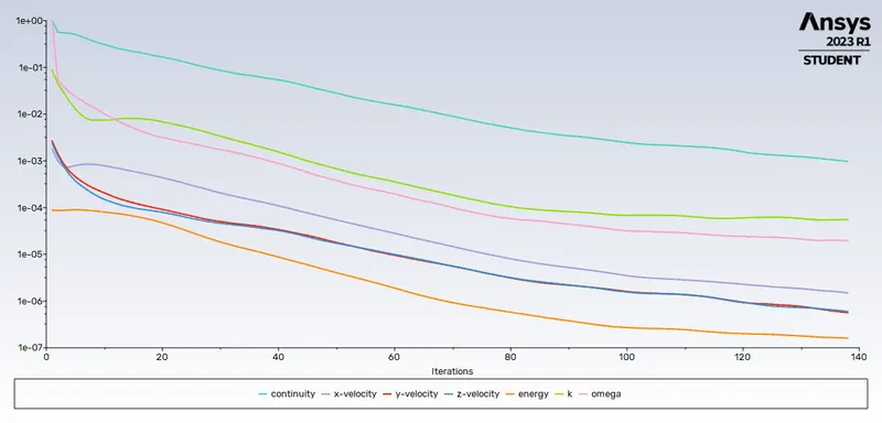
Velocity magnitude is 3m/sec. - Scaled Residuals
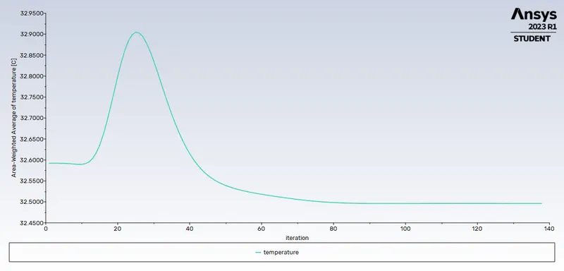
- Temperature
- Standard Deviation
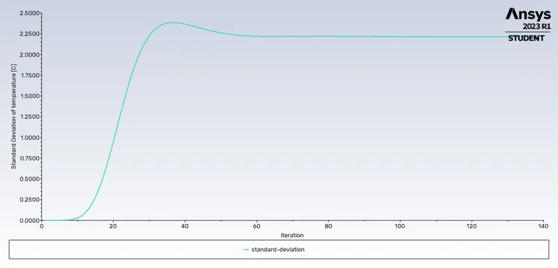
- Compute Calculation
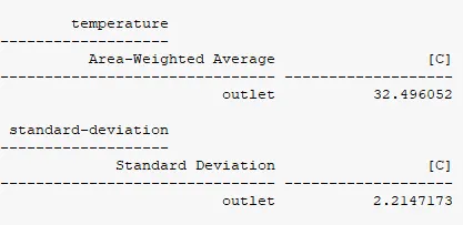
- Boundary Condition
- Post Processor Result
- Temperature Plane
- Circular
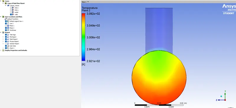
- Chart
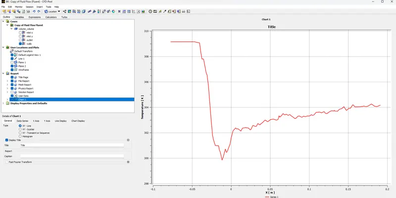
- Temperature Plane
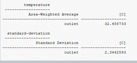
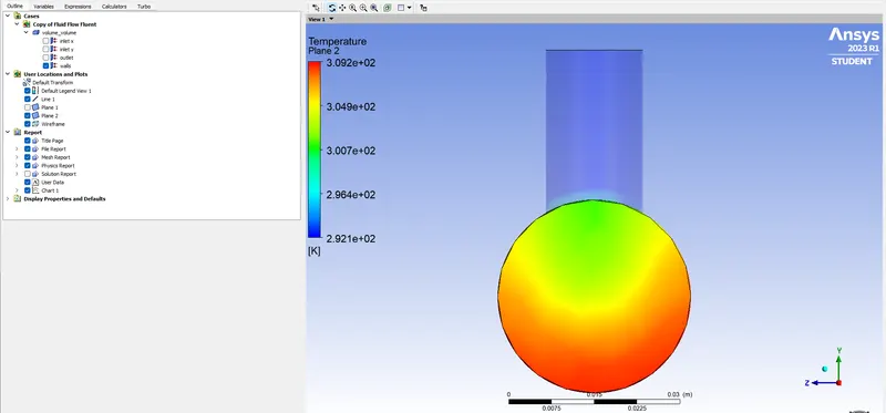
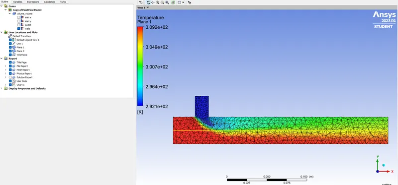
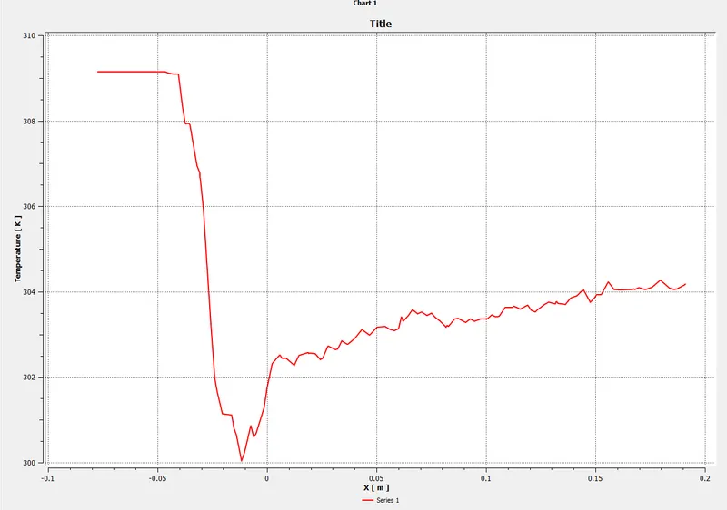
- Post Processed result of K-Omega hot inlet velocity of 6m/s. Momentum ratio of 2.
- Boundary Condition
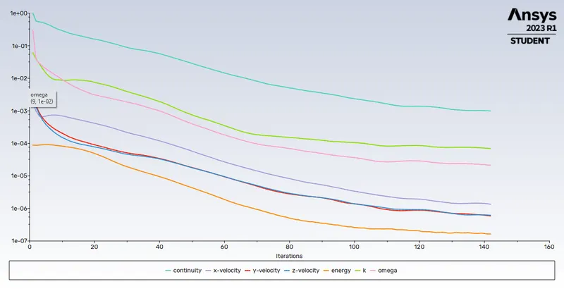
Velocity magnitude is 6m/sec. - Scale Residuals
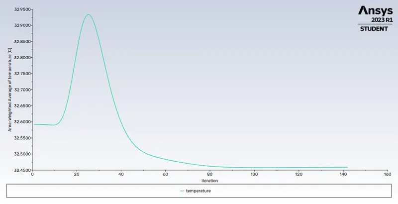
- Temperature
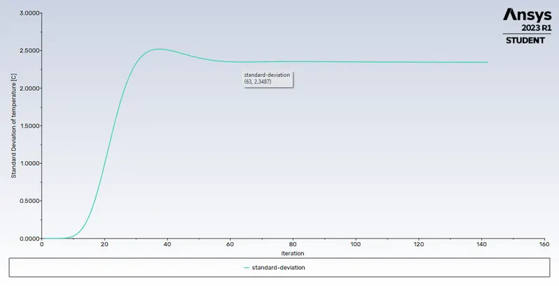
- Standard Deviation
- Compute Calculation
- Boundary Condition
- Post Processor Result
- Temperature
- Circular Plane
- Chart
- Temperature
- Post Processed result of K-Omega hot inlet velocity of 12m/s. Momentum ratio of 4.
- Boundry Condistion
Velocity magnitude is 12m/sec. - Scale Residuals
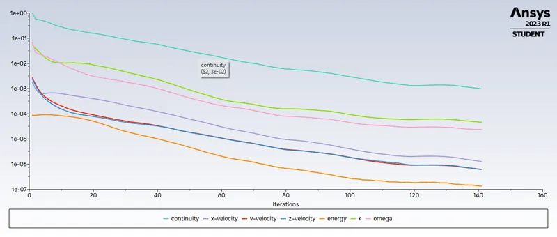
- Temperature
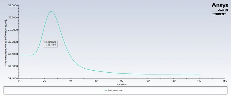
- Standard Deviation
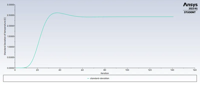
- Compute Calculation
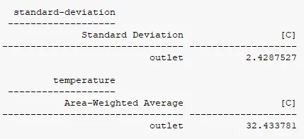
- Boundry Condistion
- Post Processor Result
- Temperature
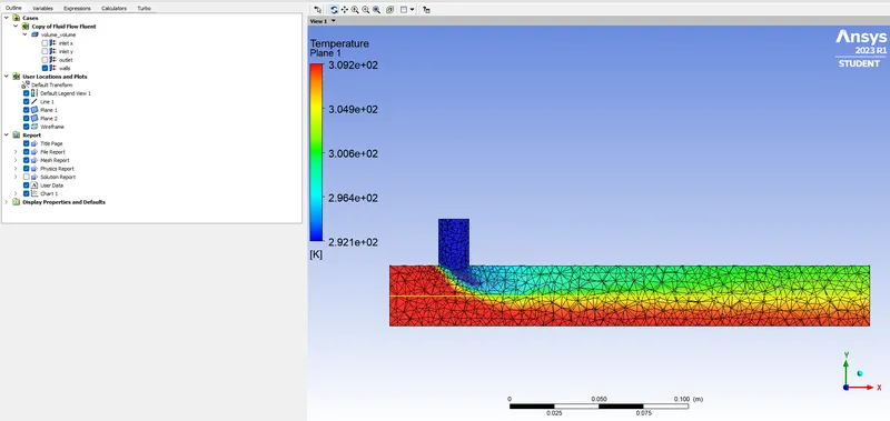
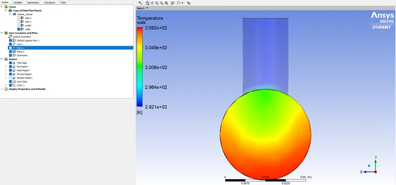
- Circular Plane
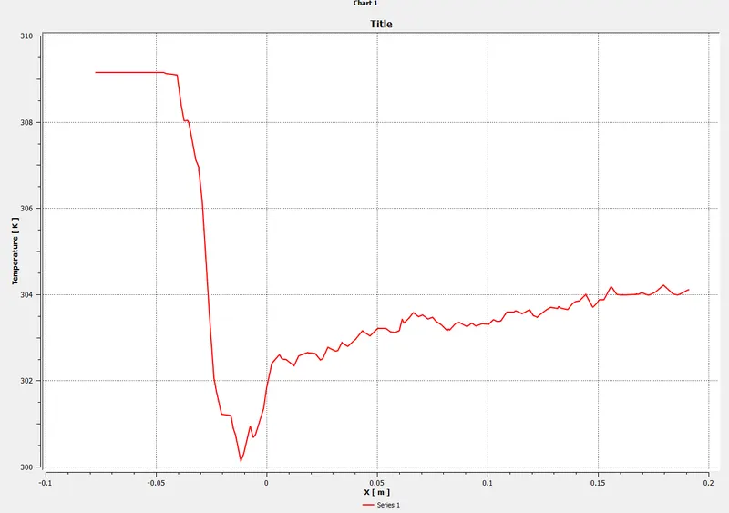
- Chart
- Temperature
Case 2
- Post Processed result of K-Epsilon hot inlet velocity of 3m/s.
- Boundary Condition
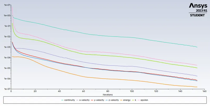
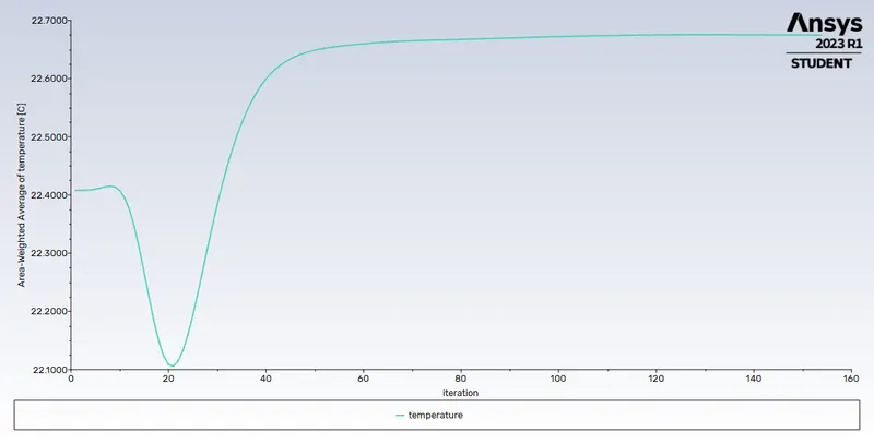
Velocity magnitude is 3m/sec. - Scale Residuals
- Temperature
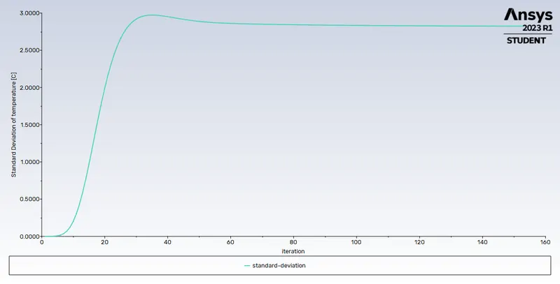
- Standard Deviation
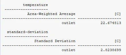
- Compute Calculation
- Boundary Condition
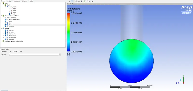
- Post Processor Result
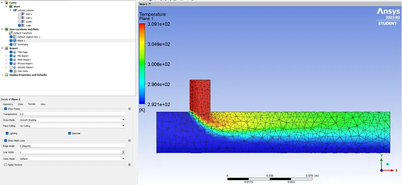
- Temperature
- Circular Plane
- Chart
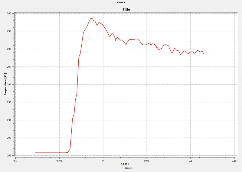
- Temperature
- Post Processed result of K-Epsilon hot inlet velocity of 6m/s. Momentum ratio of 2.
- Boundary Condition
Velocity magnitude is 6m/sec. - Scale Residuals
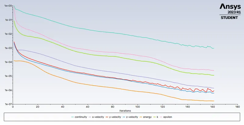
- Temperature
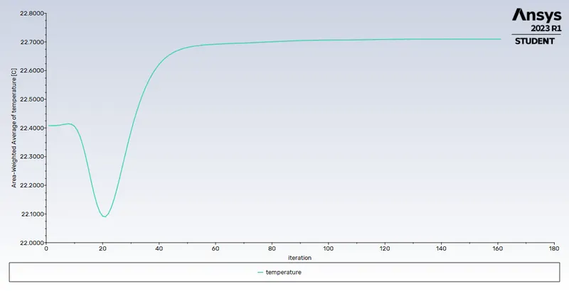
- Standard Deviation
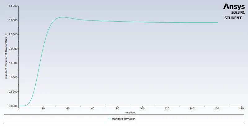
- Compute Calculation
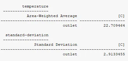
- Boundary Condition
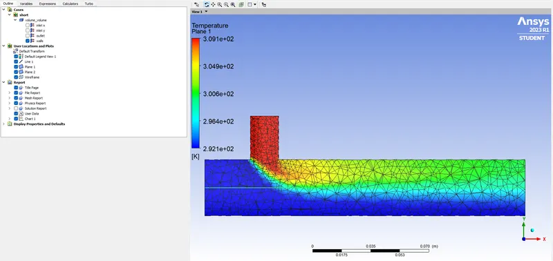
- Post Processor Result
- Temperature
- Circular Plane
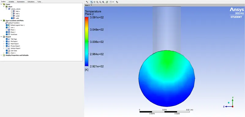
- Chart
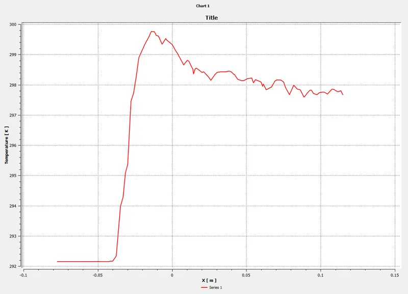
- Temperature
- Post Processed result of K-Epsilon hot inlet velocity of 12m/s. Momentum ratio of 4.
- Boundary Condition
Velocity magnitude is 12m/sec. - Scale Residuals
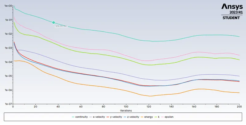
- Temperature
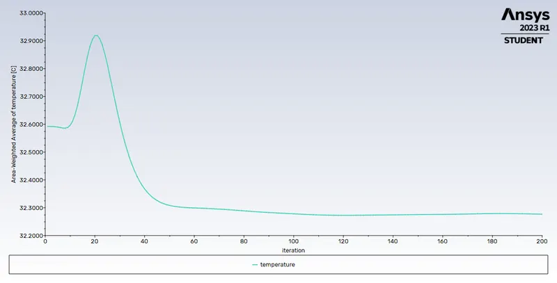
- Standard Deviation
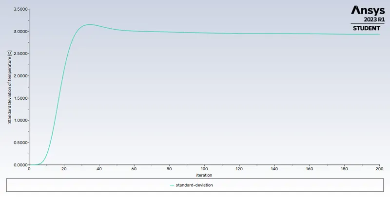
- Compute Calculation
- Boundary Condition
- Post Processor Result
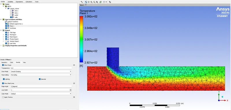
- Temperature
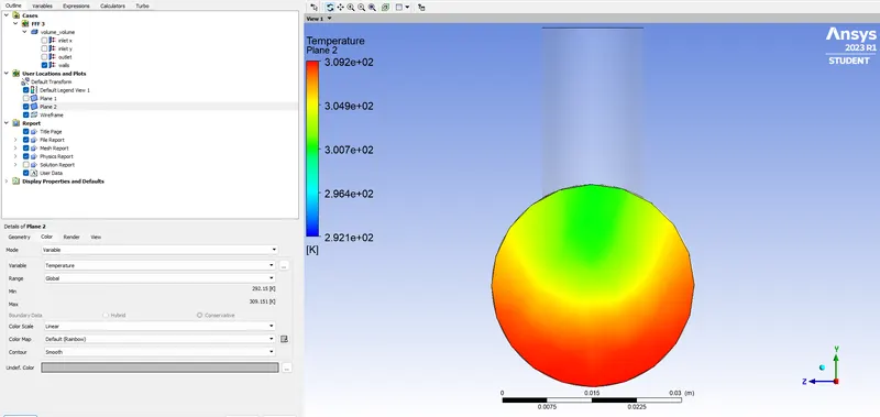
- Circular
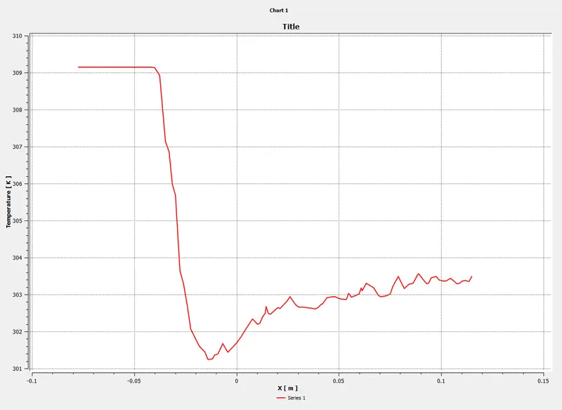
- Chart
- Temperature
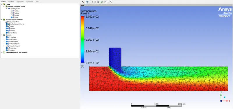
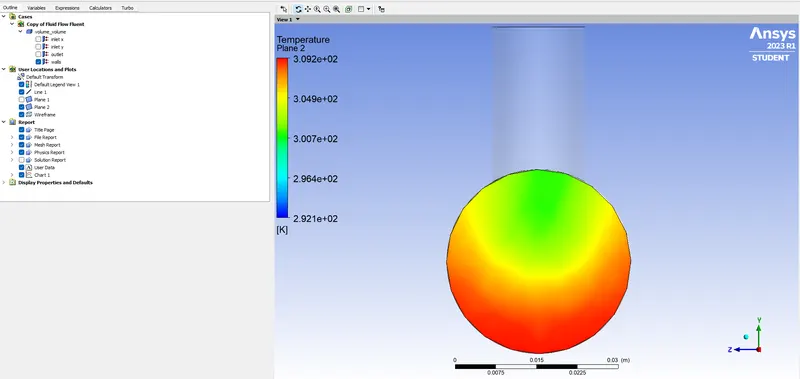
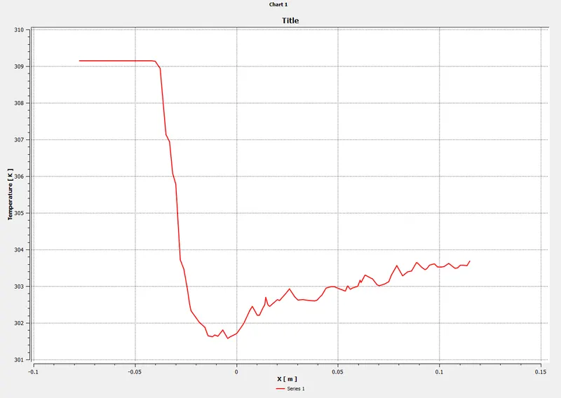
- Post Processed result of K-Omega hot inlet velocity of 3m/s.
- Boundary Condition
Velocity magnitude is 3m/sec. - Scale Residuals
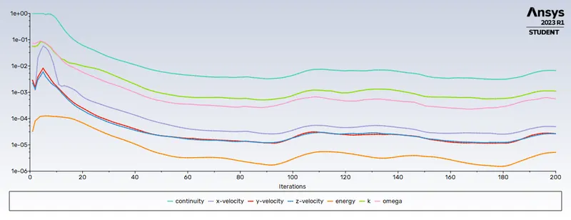
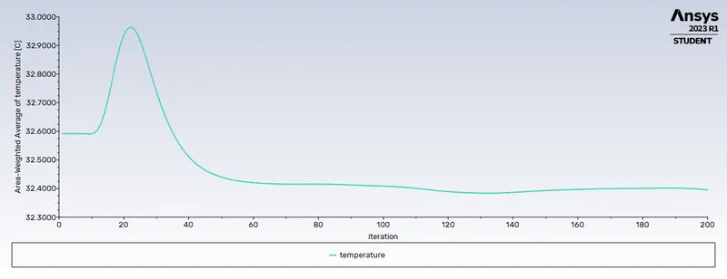
- Temperature
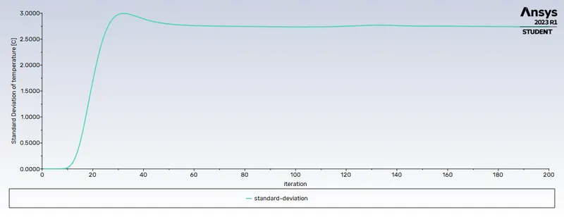
- Standard Deviation
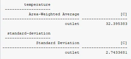
- Compute Calculation
- Boundary Condition
- Post Processor Result
- Temperature
- Circular
- Chart
- Temperature
- Post Processed result of K-Epsilon hot inlet velocity of 6m/s. Momentum ratio of 2.
- Boundary Condition
Velocity magnitude is 6m/sec. - Scale Residuals
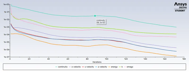
- Temperature
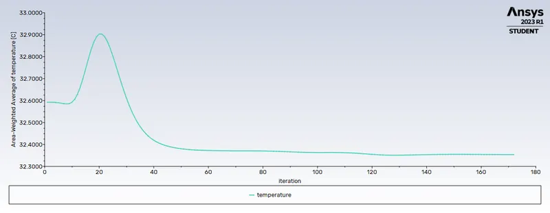
- Standard Deviation
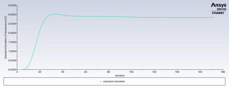
- Compute Calculation
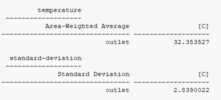
- Boundary Condition
- Post Processor Result
- Temperature
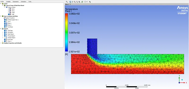
- Circular
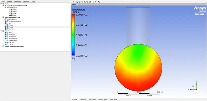
- Chart
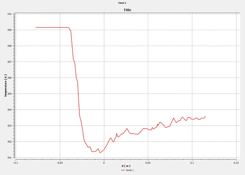
- Temperature
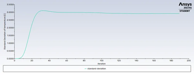
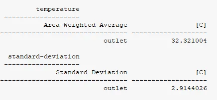
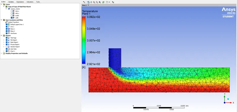
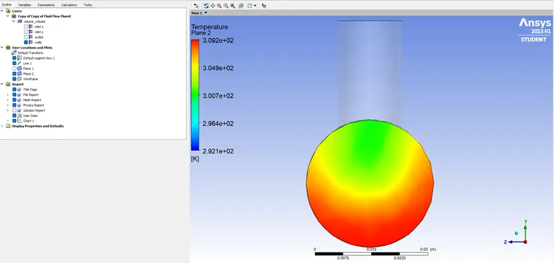
- Post Processed result of K-Epsilon hot inlet velocity of 12m/s. Momentum ratio of 4.
- Boundary Condition
Velocity magnitude is 12m/sec. - Scale Residuals
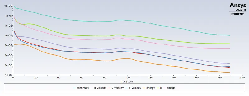
- Temperature
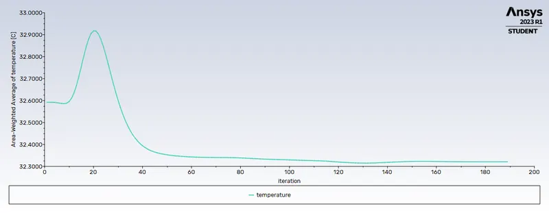
- Standard Deviation
- Compute Calculation
- Boundary Condition
- Post Processor Result
- Temperature
- Circular
- Chart
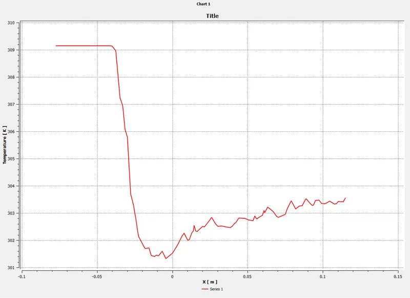
- Temperature
Result
- Fine mesh count is 221300.
- The Number of iterations is 200.
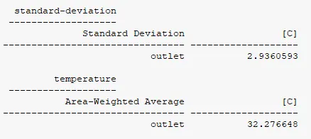
- Average outlet temperature is 31.40.
- Average standard deviation is 2.50.
Conclusion:
- The flow in a mixing tee geometry was simulated successfully using Ansys Fluent Software.
- The flow in a mixing tee geometry was also calculated analytically for the comparison with the computational results.
- The wet region (fluid flowing region) was extracted and the regions were named successfully. Once the naming is done the geometry is meshed under certain parameters and finally the case is set up.
- The first case is set up with K-epsilon and k-omega SST models to choose which have the most effectiveness with the analytically calculated value.
- By comparing the computational results with the analytical results, the K-epsilon model is more suitable for this type of simulation as this flow doesn't involve boundary layer or surface phenomenon.
- The study of flow in short mixing tee and long mixing tee have no difference in the outlet velocity and temperature. This means that the change in the length of the pipe should not affect the mixing of the flow.
- The cold stream velocity from the inlet-y creates an impact on the outlet temperature. If the velocity is increased in the inlet-y the temperature decreases significantly.
- From the mesh independent study we could observe that if we use a coarse mesh, the computational time is getting lower but when we compare the results with the finer mesh and analytical value we could observe a lot of change in the value.
- The contour plots along the pipe and across the pipe were displayed. The temperature and velocity plot along and across the pipe was also displayed.