Week 1- Mixing Tee

eAim:

• To set up steady-state simulations to compare the mixing effectiveness when the hot inlet temperature is 36 C, and the cold inlet is 19 C.
• To compare the k-epsilon and k-omega SST models for the first case to get proper judgment about each method.
• Simulate each case for the given velocity and momentum ratio.
• Compare results from the 2 cases about cell count, average outlet temperature, and the number of iterations for convergence.

Objective:

• Open the Ansys workbench and set up a fluent simulation setup, and rename it accordingly.
• Open space claims, a fluid setup, and loading the geometry.
• Identify the working fluid region in the loaded geometry and run the simulation there. Close the space claim after that.
• Next, specify boundary names for each surface in the mesh setup before creating a mesh for the fluid flow volume. Update the mesh after closing the mesh setup.
• Provide all the necessary parameters for the simulation in the setup section later on, including the simulation type, input velocity and temperature, materials (working fluid), and other user-defined parameters.
• Learn about the k-epsilon and k-omega SST concepts in setup parameters and determine which is best for the current simulation.
• After that, simulate our problem setup to determine how many iterations are necessary for our results to converge.
• Close the setup after that and update it. To view, all of the simulated results, open the results section.
• Results for each case's cell count, average outlet temperature, and convergence iteration count were generated by Combine.
• Study the effect of length and momentum ratio on the results of each case.

Introduction:

Computational fluid dynamics is a branch of fluid mechanics, which uses mathematics, physics and computational software to visualize how fluid flows and affects its medium and its neighbours. In CFD mostly computers are used to predict the fluid flow phenomena based on some governing equations like conservation of momentum – Navier stokes equation, conservation of energy etc. In this study, we are going to simulate the effect of fluid using Ansys fluent software. Ansys fluent is a very important tool in the CAE domain, which allows you to perform all three major steps of any simulation pre-processing, solving and post-processing. Ansys fluent facilitates for modeling flow, turbulence, heat transfer and chemical reactions. With Ansys, we can accomplice more in less time and with less training.

Mixing tee is a device which uses specifically engineered internal geometry to mix two fluid streams into one steam, efficiently. In this study, we are going to find the effectiveness of mixing tee. Hot air and cold air are going to be mixed in a mixing tee. They will have different velocities. We will use two different mixing tees distinguished with length and analyse the effect of length on mixing.

Short mixing tee

a - Simulation-1

hot Inlet velocity - 3 m/s

Momentum ratio - 4

b - Simulation-2

hot Inlet velocity - 3 m/s

Momentum ratio - 2

Long mixing tee

a - Simulation-3

hot Inlet velocity - 3 m/s

Momentum ratio - 4

b - Simulation-4

hot Inlet velocity - 3m/s

Momentum ratio - 2

where Momentum ratio = velocity at cold inlet/velocity at hot inlet.

Procedure:

• The study of the mixing process of tee junction using k-omega SST for Moment ratio 2 & 4. Here, we are going to use the same geometry and mesh for both cases of simulation.
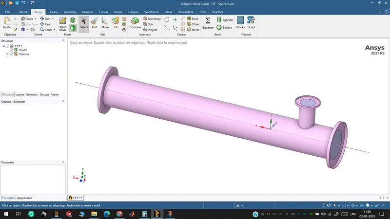
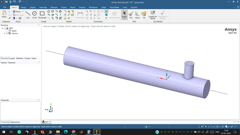
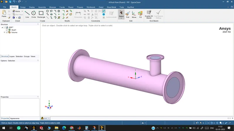
• The geometry of the long tee and short tee is shown below.

Long Mixing tee

Short Mixing tee:

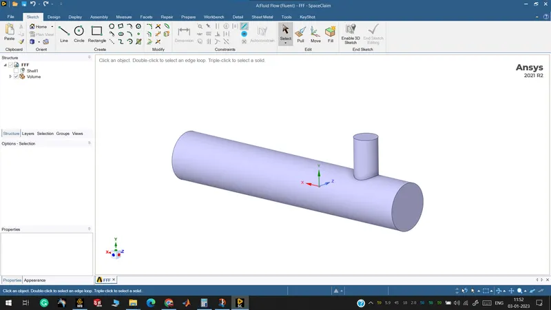
• We are to analyze the mixing of two fluids, so there is a role of parts other than two pipes. To suppress that we need to extract the volume of a tee. Go to prepare the menu and click on volume extract. Switch to edge selection and select three outer edges and click on the green check button. Hide solid by unchecking it from the structure menu to see the volume, which we have extracted. Suppress solid by clicking on the option suppress for physics. Exit from Spaceclaim and click on the mesh to open the mesh menu.

• Now, we can go for meshing. where we can generate the mesh and provide names for all the surfaces of the geometry.

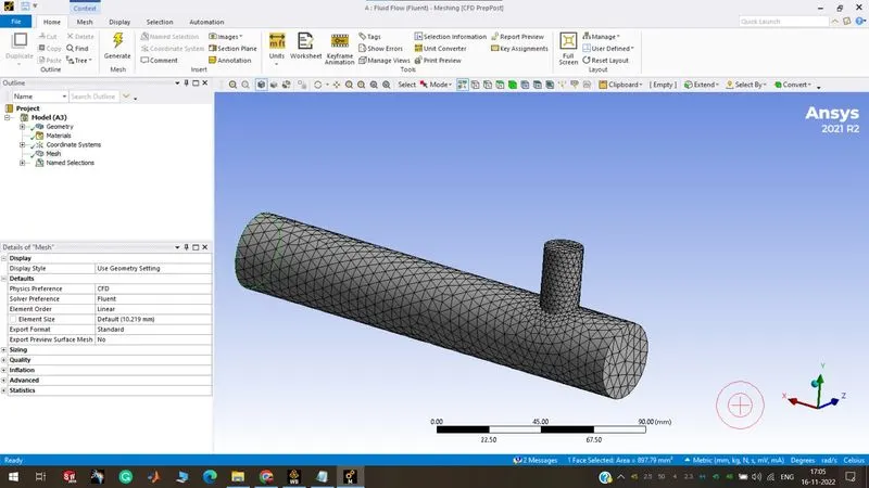
• As you can see the default mesh is generated. Where this mesh has the default mesh element size which leads to bad results and less accuracy.

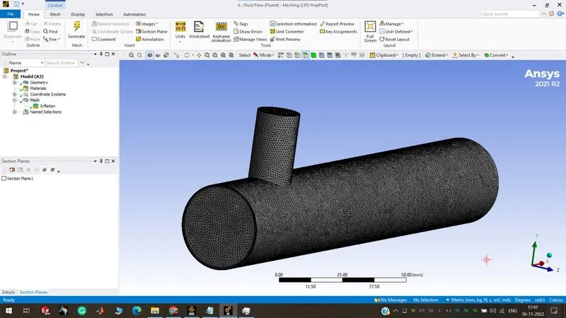
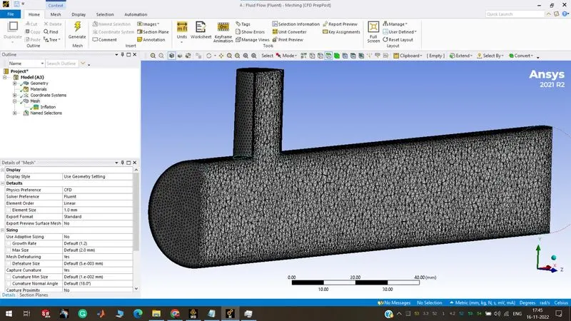
• Now, the above images are shown with a clear understanding of mesh independent study. As the mesh element size is 1mm with 10 layers of inflation of the max thickness of 1mm.
• Now, In the fluent tab, we will be setting up all the parameters which are required.
• where in the step-up tab, the pressure-based solver is used with steady-state analysis. And SST-K-omega viscous model is used and taking air as default with 1.225kg/m3 density.
• Boundary conditions as (a)inlet_-_x (b) inlet_-_y (c)outlet (d) walls
• 
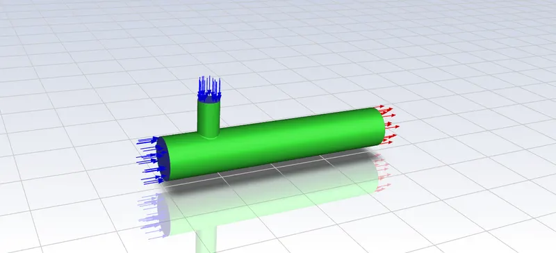
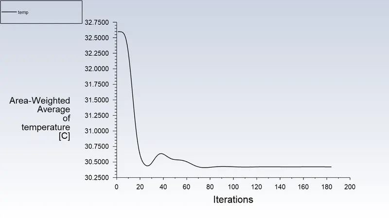
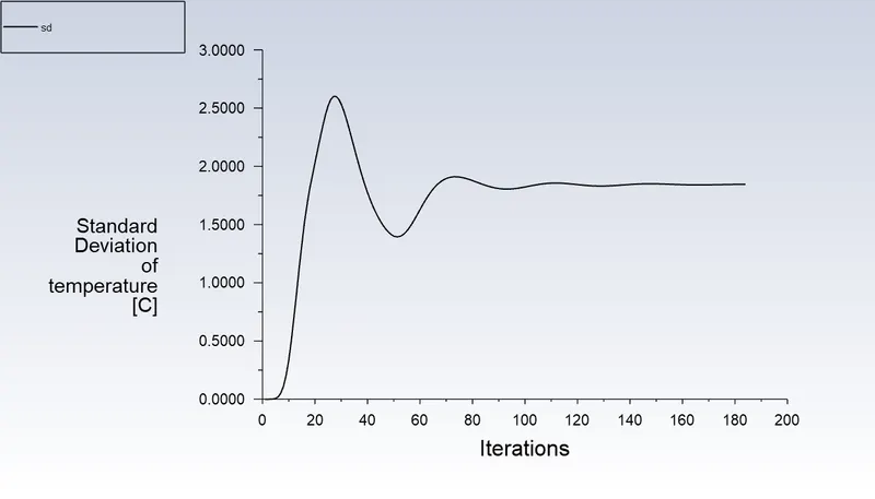
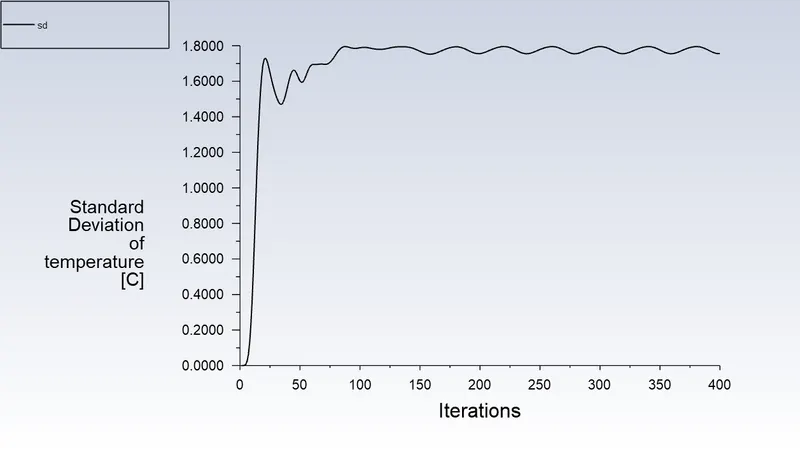
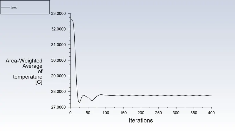
• Calculating the area-weighted average and standard deviation at the outlet as temperature.
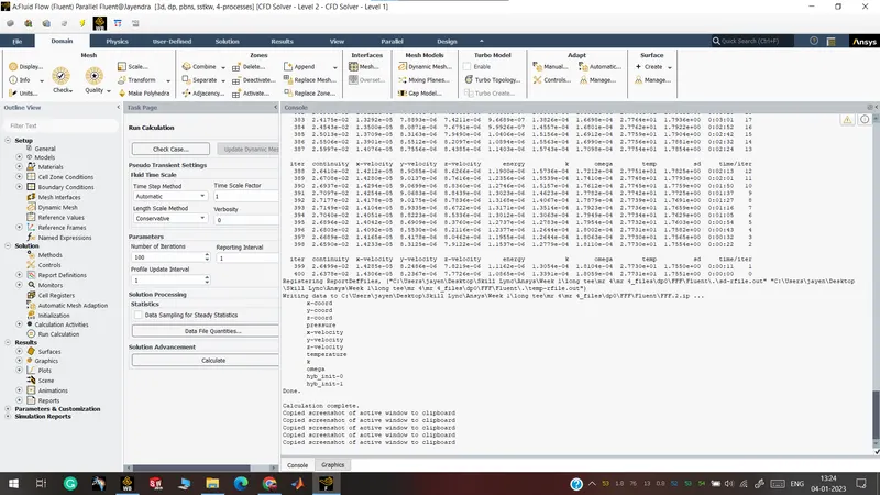
• And initialization with hybrid mode to get better results with 200 iterations.

Results:

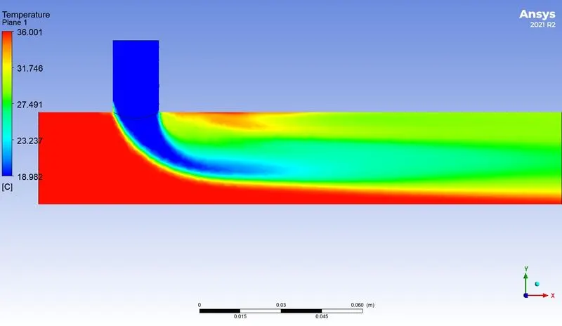
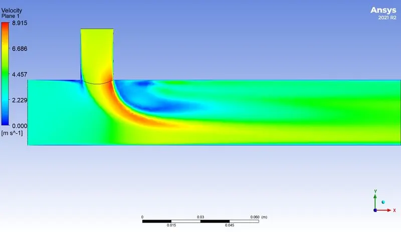
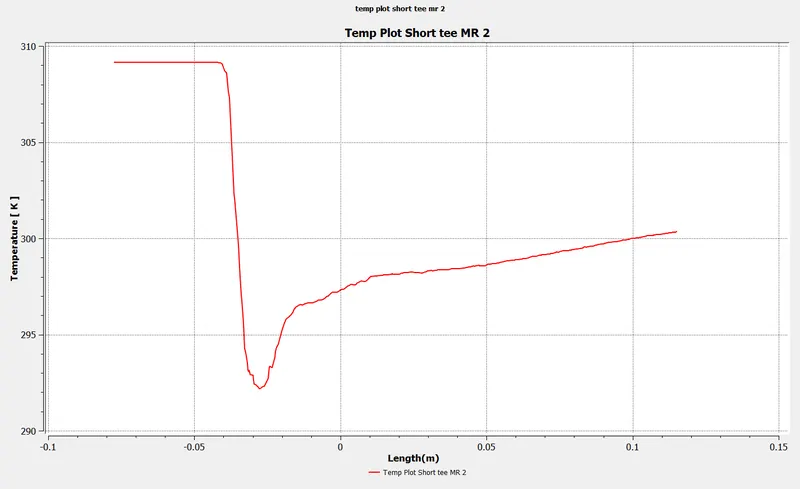
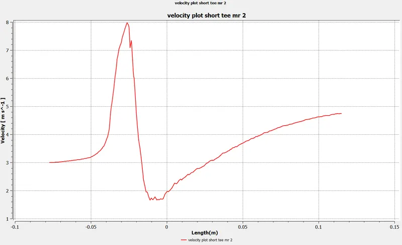
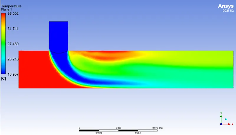
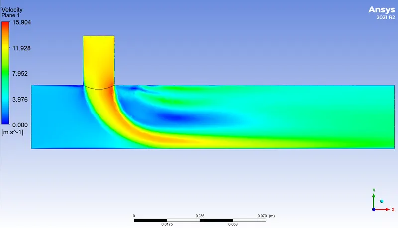
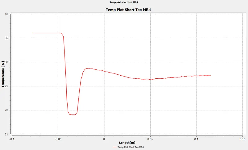
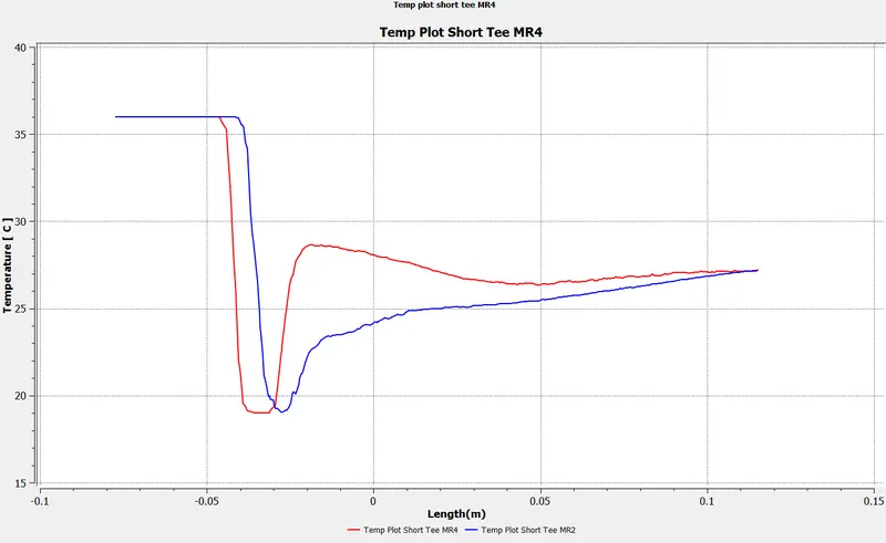
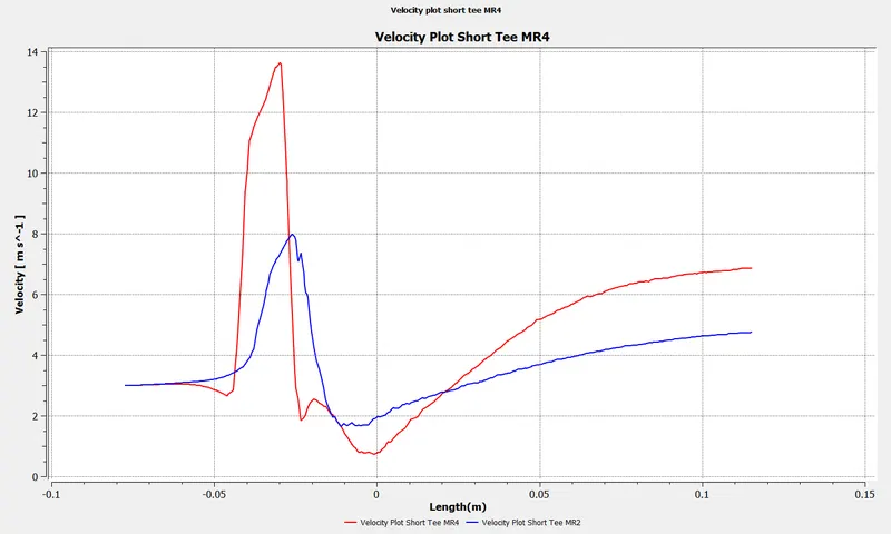
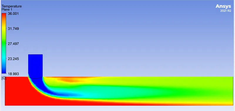
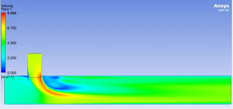
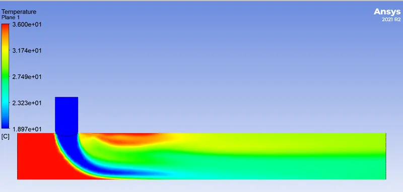
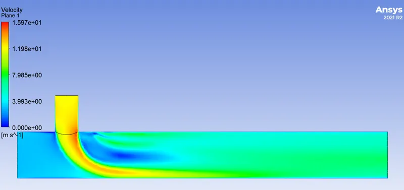
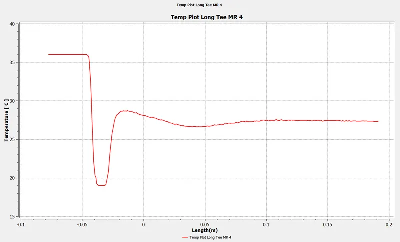
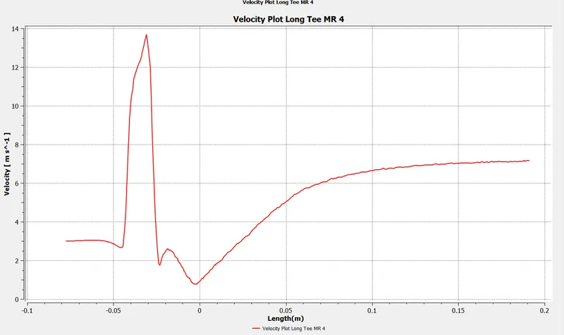
After the simulation of the mesh elements, we will get some temperature and velocity which changes with respect to factors like velocity, length of pipe, mesh element sizes, etc. we will discuss both the cases on the fluctuation of temperature and velocity below images present the temperature and velocity profile for the different conditions.

Short tee mixing :

Moment Ratio 2:

short tee mr2 Temperature:

short tee mr2 velocity:

Plots

MR 2 Temperature plot

MR 2 Velocity plot

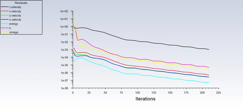
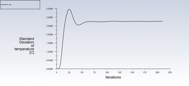
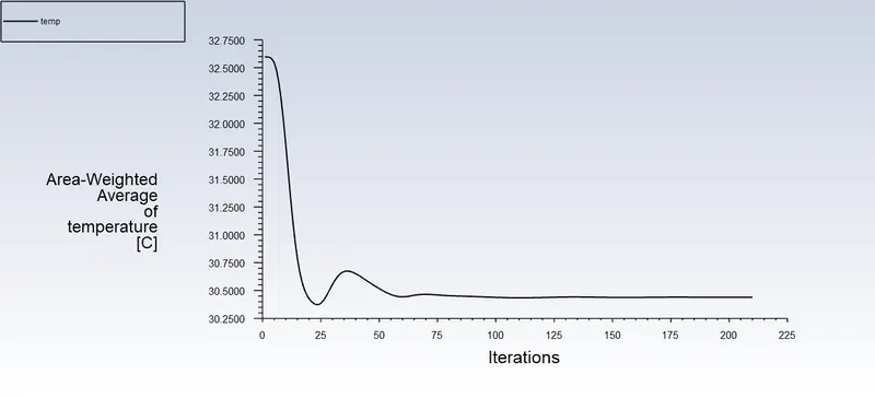
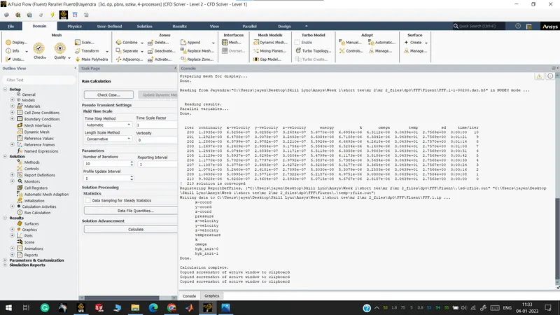
Moment Ratio 4:

Temperature contour

Velocity

Plots

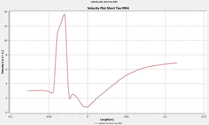
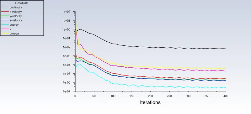
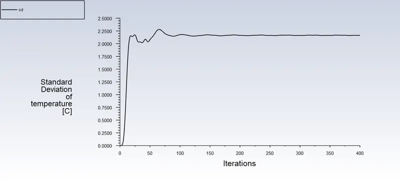
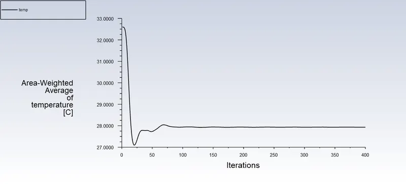
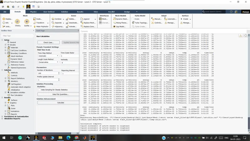
Comparison of both Moment ratios 2 & 4 for short tee

Sr no	Cases	Avg Outlet temp(K)			Cell count	No.of Iteration for convergence of solution
		Theoretically		Numerically
1	ST with MR=2	303.52	303.59		1119207	210
2	ST with MR=4	300.23	301.08		1119207	400

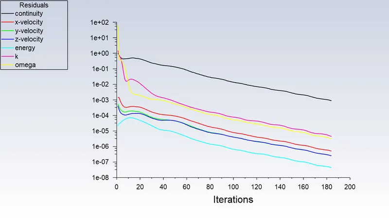
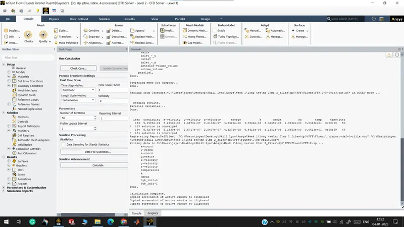
Long Tee mixing:

Temperature Plot Long Tee MR 2

Velocity Plot Long Tee MR 2

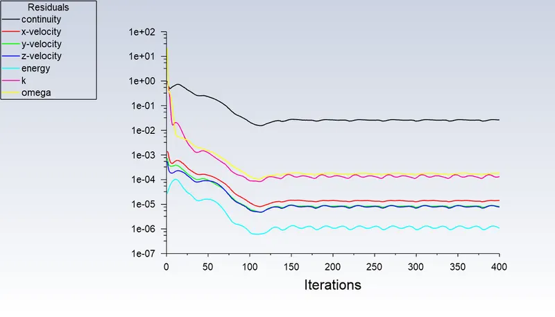
MR 4

Sr no	Cases	Avg Outlet temp(K)			Cell count	No.of Iteration for convergence of the solution
		Theoretically		Numerically
1	LT with MR=2	303.52	303.57		1516437	184
2	LT with MR=4	300.23	300.88		1516437	400

Conclusion

In the above analysis, we are able to know how the temperature in the mixing tee is act with respect to the velocity and length of the pipe. Velocity will be different in the different regions which very much fluctuates near the wall which is equal to zero it gradually increases with increasing height; at these places, the heat transfer takes place more. In the mixing line of hot and cold air temperature is fluctuate.

We are using the k-omega-sst model to solve the problem which gives a more accurate result in this condition. In the result and discussion, we are able to know much more about how the mesh and other parameters affect the result which is outlet temperature. In the analysis, we can see how the temperature and velocity profile is given. In the turbulence mixing of the model in the T junction, the temperature is defined from the RANS model and it is also compared with the SST model. In our two cases use the RANS model because the SST model gives more different from the RANS model.

Link:

https://drive.google.com/drive/folders/1imxs1k6ZqvEfWfYPJcTbkPjArcjWehZR?usp=sharing