Week 1- Mixing Tee

MIXING TEE

AIM: To create two versions of the longer and short mixing tee.

OBJECTIVE:

• To set up steady-state simulations to compare the mixing effectiveness when hot inlet temperature is 36⁰C & the Cold inlet is at 19⁰C.
• Use k-epsilon and k-omega SST model.
• Case 1
• Short mixing tee with a hot inlet velocity of 3m/s.
• Momentum ratio of 2, 4.
• Case 2
• Long mixing tee with a hot inlet velocity of 3m/s.
• Momentum ratio of 2, 4.

THEORY AND EXPLANATION:

Computational fluid dynamics is a branch of fluid mechanics, which uses mathematics, physics and computational software to visualize how fluid flows and affects its medium and its neighbors. In CFD mostly computers are used to predict the fluid flow phenomena based on some governing equations like conservation of momentum – Navier stokes equation, conservation of energy etc. In this study we are going to simulating effect of fluid using Ansys fluent software. Ansys fluent is a very important tool in CAE domain, which is allows you to perform all the three major steps of any simulation pre-processing, solving and postprocessing. Ansys fluent facilitates for modelling flow, turbulence, heat transfer and chemical reactions. With Ansys we can accomplice more in less time and with less training.

Mixing tee is a device which uses specifically engineered internal geometry to mix two fluid streams into one steam, efficiently. In this study we are going to find effectiveness of mixing tee. Hot air and cold air are going to be mixed in mixing tee. They will have different velocities. We will use two different mixing tee distinguished with length and analyze the effect of length on mixing.\

CASE setup-

Pre-processing- SpaceClaim.

The CAD model is imported into the SpaceClaim to extract the flow volume field from the model. The extracted volume is shown below:

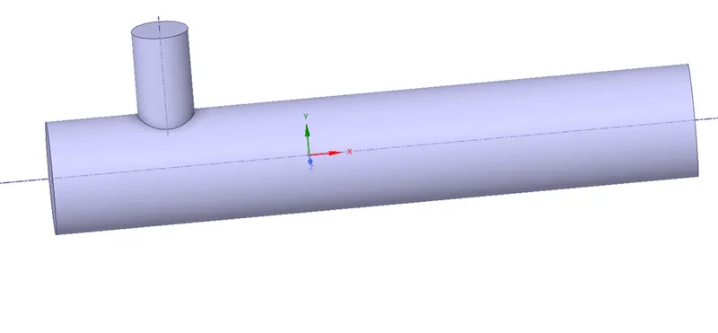
Fig. a

Mesh

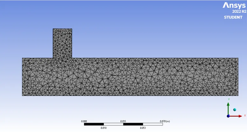
The boundary names are applied in this section and a mesh is generated.

Setup

In this section, we apply different boundary conditions like inlet, outlet boundary conditions. Turbulence models are set up like K-epsilon or K-omega for solving the turbulent mixing of air. The number of iterations is set in this section.

Solution

In this section the setup already solved the by creating plots for area-weighted volume, standard deviation of temperature, area-weighted temperature as well as residual plot.

CFD-Post

Post-processing is carried in this section in which different contours are setup to visualize the properties (such as Temperature, velocity etc.) for which simulation is run.

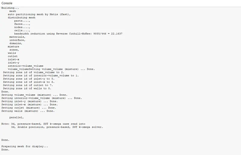
Fig. b

CASE 1- SHORT TEE

a) For inlet velocity of 3m/s and momentum ratio of 2

Mesh size- 0.003 m

A mesh element metric that identifies the quality of mesh was employed and it can be seen that the elements of the lowest quality are minimal. Most of the elements have quality in the range of 0.7-1. Hence, the mesh is of acceptable quality.

Fig.1.1

Mesh: The number of elements is 39,725

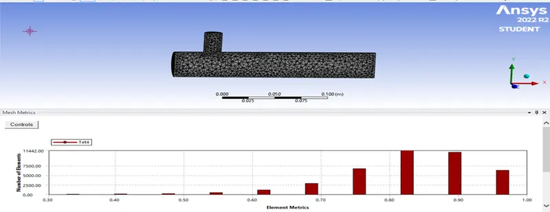
Fig.1.2

RESIDUAL PLOT:

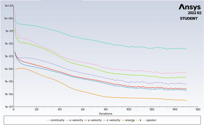
Fig. 1.3

STANDARD DEVIATION:

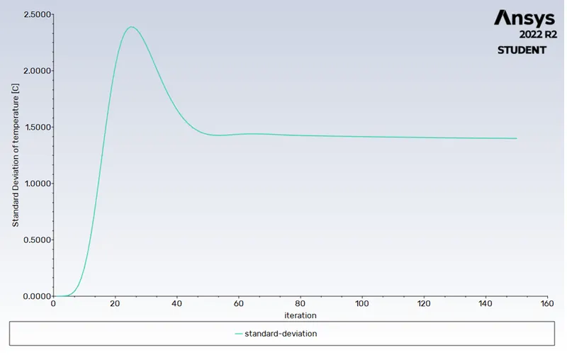
Fig. 1.4

TEMPERATURE:

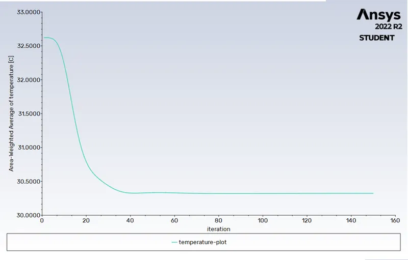
Fig. 1.5

VELOCITY:

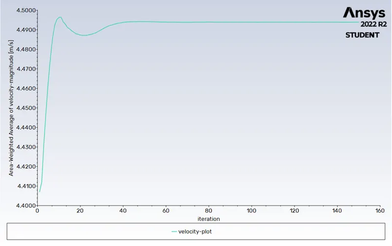
Fig. 1.6

CONTOURS:

1. Temperature:

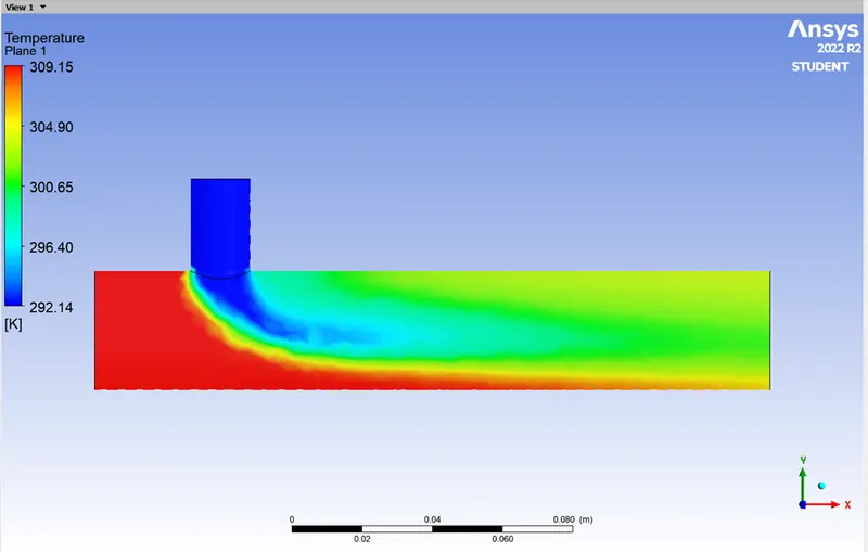
Fig. 1.7

2. Velocity:

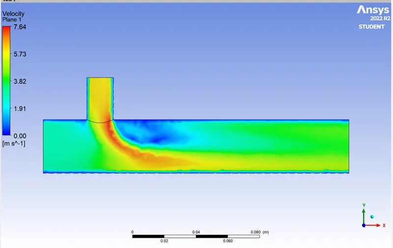
Fig. 1.8

b) For inlet velocity of 3m/s and momentum ratio of 4

Mesh size- 0.003 m (mesh remains the same as the above case)

RESIDUAL PLOT:

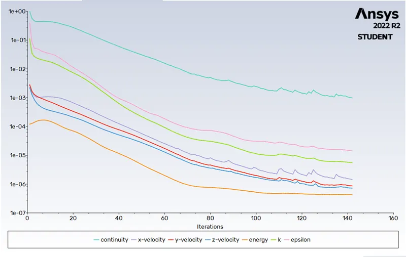
Fig. 2.1

STANDARD DEVIATION:

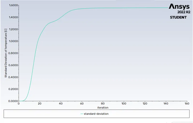
Fig. 2.2

TEMPERATURE PLOT:

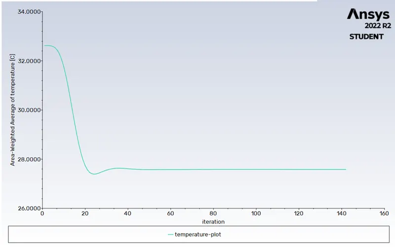
Fig. 2.3

VELOCITY PLOT:

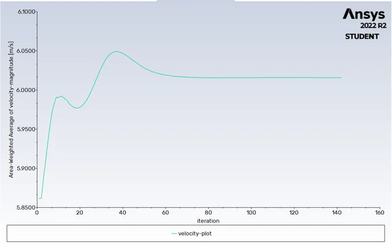
Fig. 2.4

CONTOUR :

1. Temperature:

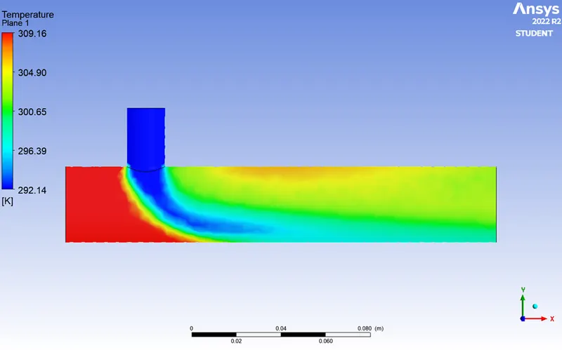
Fig. 2.5

2. Velocity Plot:

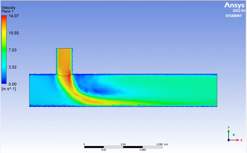
Fig. 2.6

For inlet velocity of 3m/s and momentum ratio of 2,4. From the given value the result says that the momentum ratio 2 is better than momentum ratio 4 in Short Tee model for the output plots. As the in 3D model temperature is increase slightly at outlet and the velocity at outlet is doubled as comere of case-a and case-b models.

CASE 2- LONG TEE

a) For inlet velocity of 3m/s and momentum ratio of 2

Mesh size- 0.003 m

A mesh element metric that identifies the quality of mesh was employed and it can be seen that the elements of the lowest quality are minimal. Most of the elements have quality in the range of 0.7-1. Hence, the mesh is of acceptable quality.

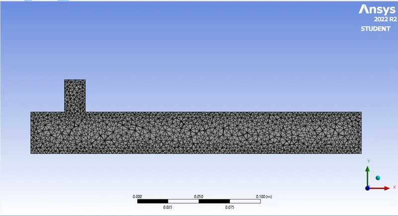
Fig. 3.1

Mesh: The number of elements is 56,670

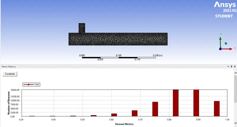
Fig. 3.2

RESIDUAL PLOT:

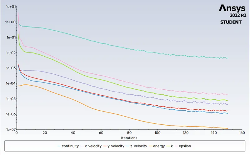
Fig. 3.3

STANDARD DEVIATION:

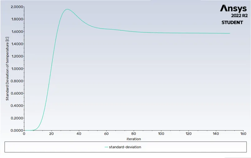
Fig. 3.4

TEMPERATURE PLOT:

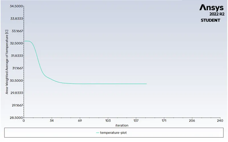
Fig. 3.5

VELOCITY PLOT:

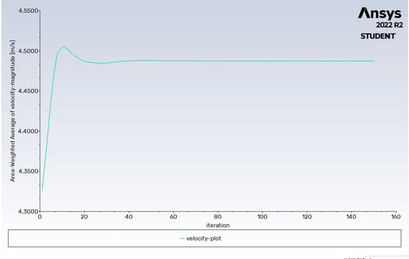
Fig. 3.6

CONTOUR:

1. Temperature

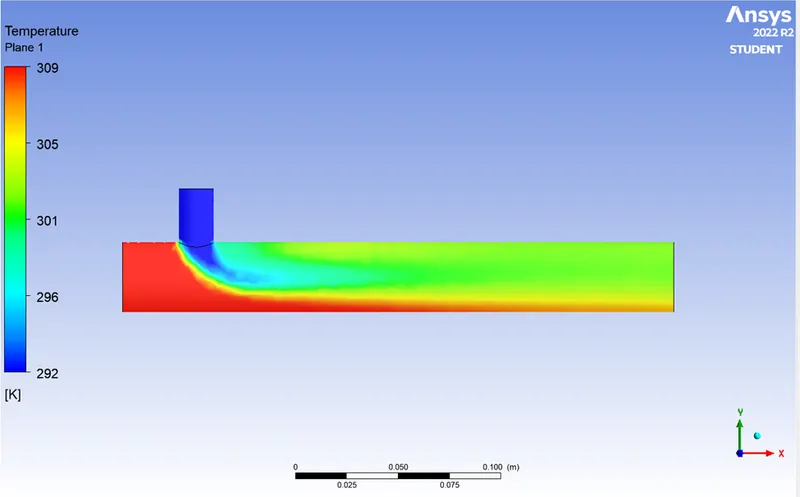
Fig. 3.7

2. Velocity

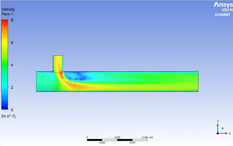
Fig. 3.8

b) For inlet velocity of 3m/s and momentum ratio of 4

Mesh size- 0.003 m (mesh remains the same as the above case)

RESIDUAL PLOT:

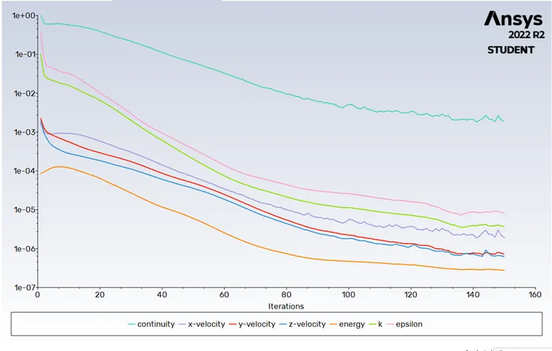
Fig. 4.1

STANDARD DEVIATION:

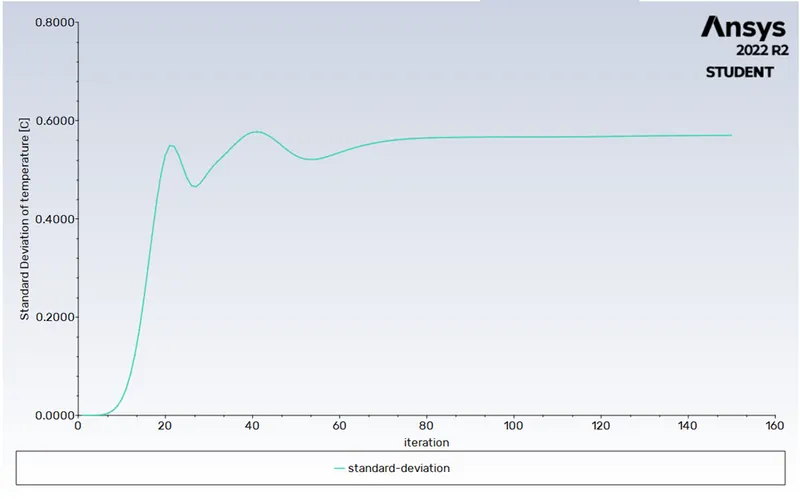
Fig. 4.2

TEMPERATURE PLOT:

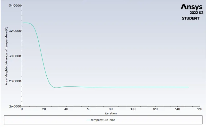
Fig. 4.3

VELOCITY PLOT:

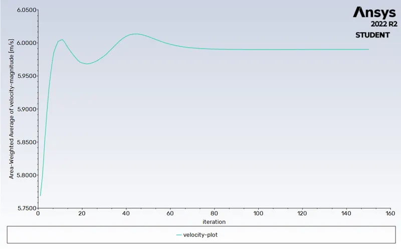
Fig. 4.4

CONTOUR:

1. Temperature:

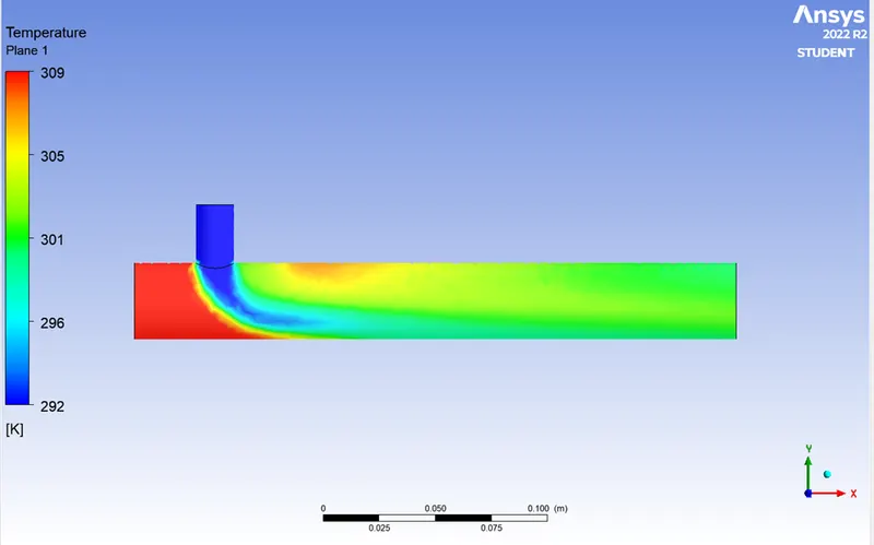
Fig. 4.5

2. Velocity:

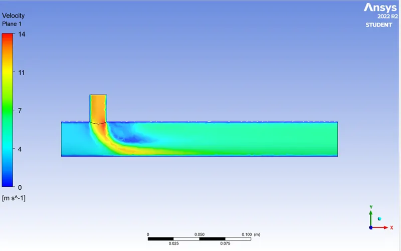
Fig. 4.6

For inlet velocity of 3m/s and momentum ratio of 2,4. From the given value the result says that the momentum ratio 2 is better than momentum ratio 4 in Long Tee model for the output plots. As the in 3D model temperature is increase slightly at outlet and the velocity at outlet is doubled as comere of case-a and case-b models.

Effect of Turbulence model:

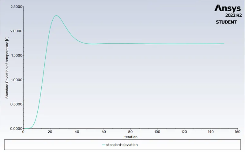
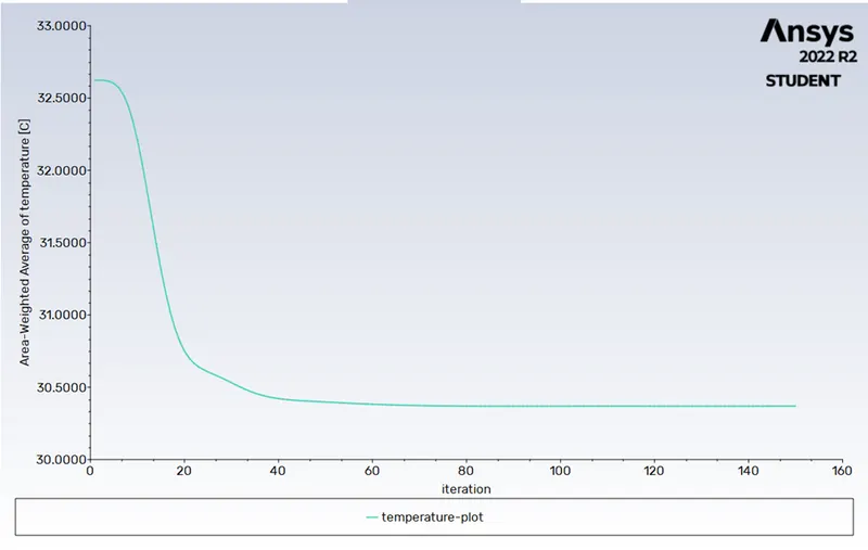
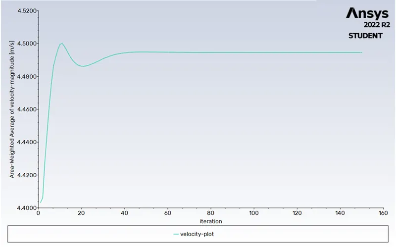
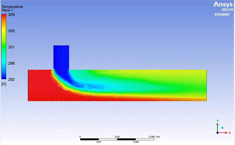
K-ω">ωSST model used for carrying out this experiment is Short TEE. Mesh remains the same as the Short tee mesh picture is visualized. The inlet velocity is 3 m/s and momentum ration is 2.

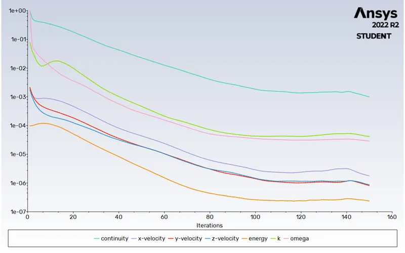
RESIDUAL PLOT:

STANDARD DEVIATION:

TEMPERATURE PLOT:

VELOCITY PLOT:

CONTOUR:

1. Temperature:

2. Velocity:

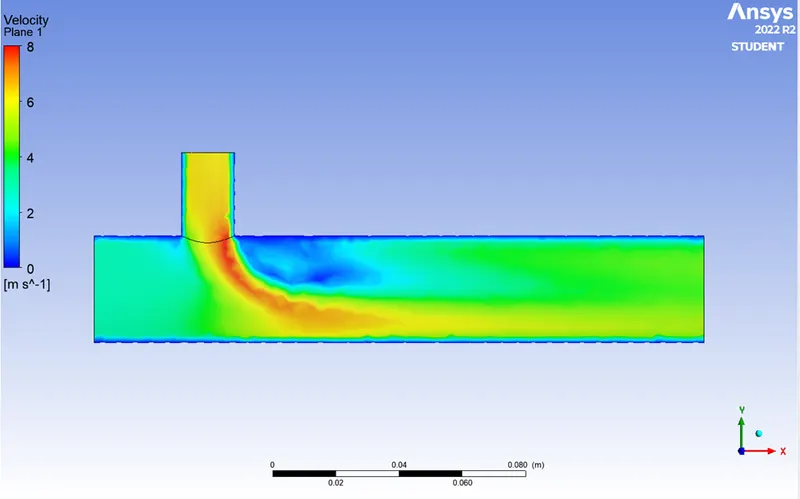
By comparing k-epsilon and k-omega the residual plot considers the smoother plot in k-omega as comare to k-epsilon at same mesh and momentum ratio of Short-Tee model.

Comparison of all cases:

Case	Cell count	Average outlet temperature (K)	Number of iterations for convergence
Short tee- Momentum ration 2	39,725	303.439	152
Short tee- Momentum ration 4	39,725	300.699	150-160
Long tee- Momentum ration 2	56,670	303.549	150
Long tee- Momentum ration 4	56,670	300.639	150-160

As compare to Lond-Tee and Short-Tee model the cell count of mesh changes but in temperature and velocity output no more changes.

Comparing in momentum ratio of 2 and 4 for both Long-Tee and Short-Tee change or more in area-weighted temperature, standard deviation and area-weighted velocity plots as well in output model.

CONCLUSION:

1. As seen in the Case-1-a and Case-1-b, the temperature at the outlet drops down significantly due to high velocity of cold air from the inlet. This is possible due to the turbulent mixing at the tee joint between hot air and cold air because of the high velocity of cold air., which is not possible in case of low-velocity cold air.
2. The temperature contour at the outlet for short tee cases shows that some of the high temperatures flow sips through without properly mixing with the flow. Whereas, in the temperature contour of long tee cases, the high temperatures flow thoroughly mixes with the rest of the flow.
3. Therefore, we can recommend using the long tee and high-velocity inlet for application. This is because we have a low standard deviation in case of long tee compared to the short tee for both momentum ratios.
4. k- epsilon model predicts well far from the boundaries (wall) and k- omega model predicts well near the wall. Even though it depends on Y+. Therefore, K-epsilon model is majorly used for free flow away from the wall and as in this project, there is no dealing with the wall of the mixing tee for change in temperature along the length of it, so K-epsilon model was chosen for further simulations.