Week 1- Mixing Tee

AIM:

Set up steady-state simulations to compare the mixing effectiveness when hot inlet temperature is 36⁰C & the Cold inlet is at 19⁰C for short and long tee.

Use the k-epsilon and k-omega SST model for the first case and based on the judgment use the more suitable model for second case of long tee. Giving the reason for choosing a suitable model is compulsory.

1. Case 1
• Short mixing tee with a hot inlet velocity of 3m/s.
• Momentum ratio of 2, 4.
2. Case 2
• Long mixing tee with a hot inlet velocity of 3m/s.
• Momentum ratio of 2, 4.

Momentum ratio = velocity at cold inlet / velocity at hot inlet

In a table, compare the following values from the 2 cases.

1. Cell count
2. Average outlet temperature
3. Number of iterations for convergence

For each simulation, show the convergence plot

OBJECTIVE:

1. Velocity and temperature contour plots on the cut planes along and across the pipe.
2. Perform Mesh independent study for any one case.

INTRODUCTION:

Mixing tee is a drafted model which typically utilize heterogeneous mixing phenomenon to increase the temperature of chilled air to that of human comfort as mentioned in ASHRAE standards.

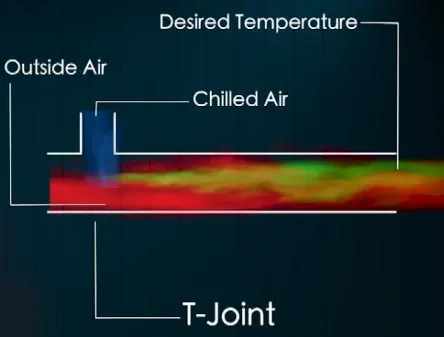
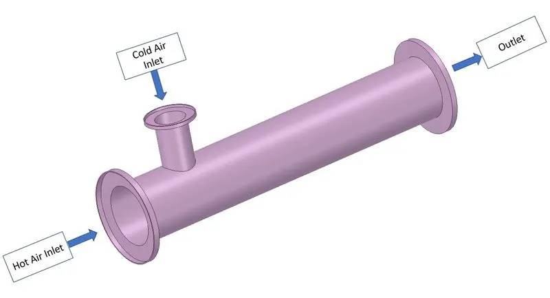
THEORY:

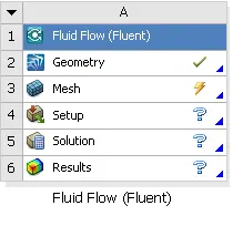
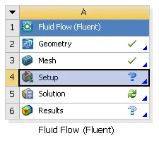
Computer uses data structures, numerical analysis and simulation to simulate free stream flow of fluid flows in accordance to real life and interaction of fluids with surfaces are captured which are defined by boundary conditions. .Here we uses Ansys CFD Simulation to visualize the effects of temperature at the outlet of mixing tee. Workflow in Ansys is given below.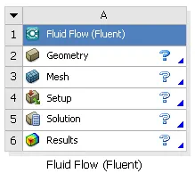

PROCEDURE:

SOLVING AND MODELLING APPROACH:

SHORT TEE MR:2

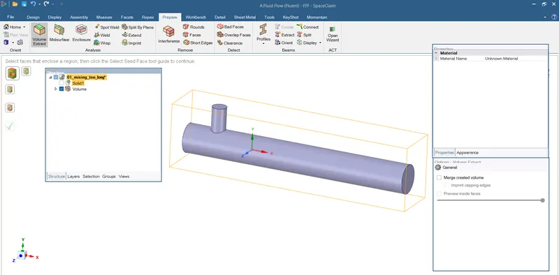
1. Open Geometry- Spaceclaim in Ansys 19.2
2. Import model and extract volume using edge selection.
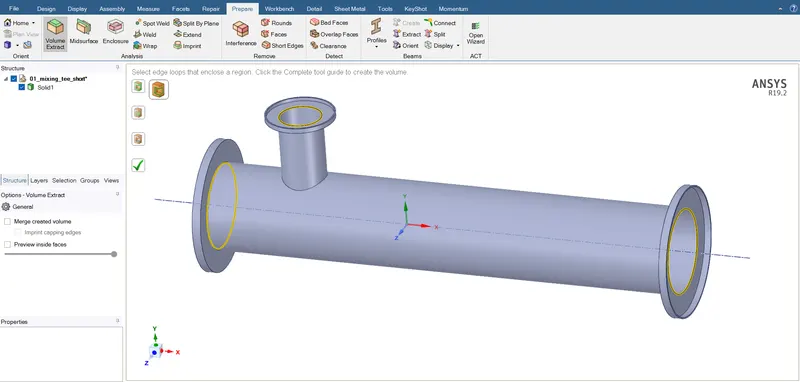
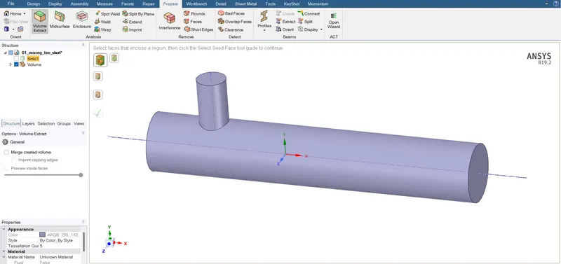
3. Supress solid body for physics

PREPROCESSING AND SOLVER SETTING:

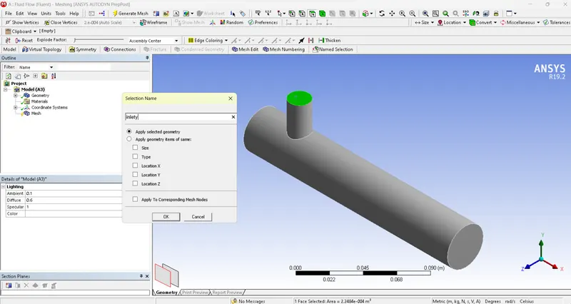
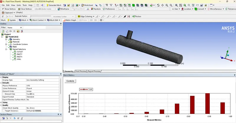
1. Open Mesh module.
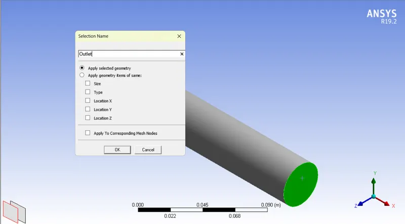
2. Give named selections for inlet in and y direction, outlet and wall faces.
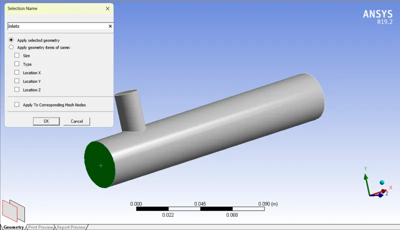
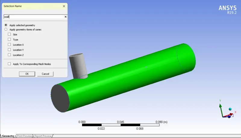
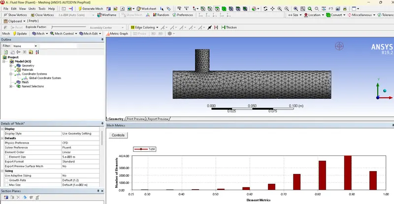
3. Set for 5mm mesh and in quality check for mesh metrics-Element quality. Here it is noted that element metrics is greater than 5%.So this is satisfiable.
4. Now moving to setup.
5. In units set temperature in deg celcius.
6. In setup domain Select solver settings to pressure based and steady state.
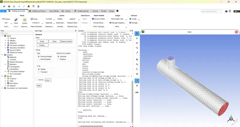
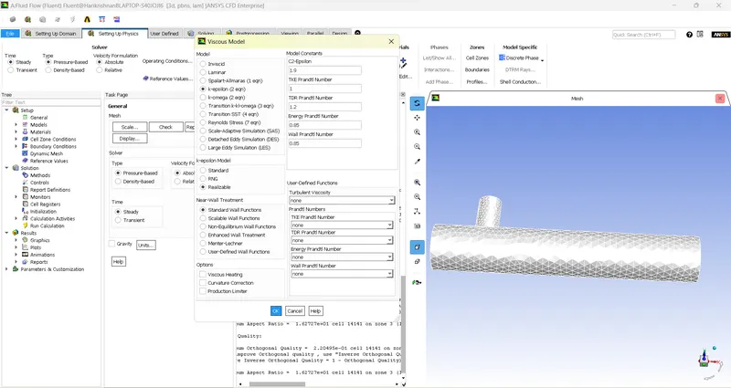
7. In setting up physics select energy and select suitable turbulence model. Here we select k-epsilon realizable model.
8. Select cell zone conditions and select fluid type to air.
9. Now select boundaries and select inlet x and velocity as 3m/s and temperature 36deg celcius.
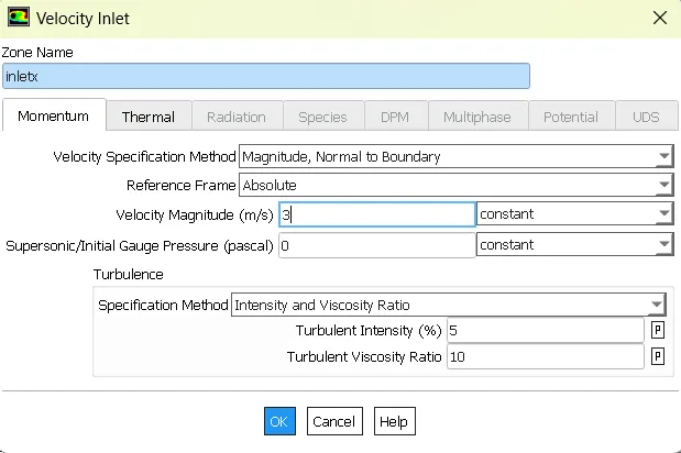
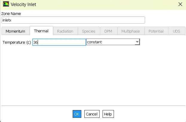
10. Now select boundaries and select inlet y and velocity as 6m/s and temperature 19deg celcius.
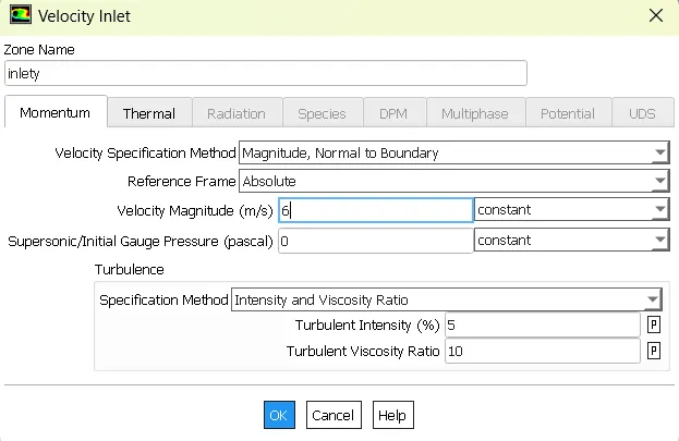
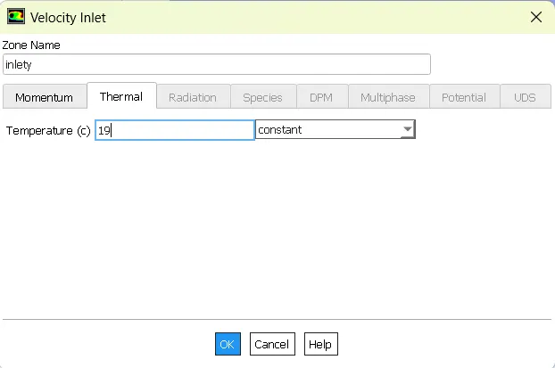
11. Now select outlet and make pressure as gauge pressure default.
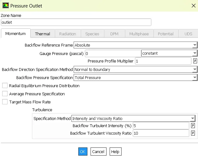
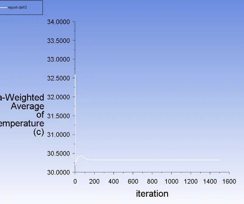
12. Now give surface report definition for area weighted average for temperature at outlet.
13. Now give surface report definition for standard deviation for temperature at outlet.
14. Now select hybrid initialization and initialize.
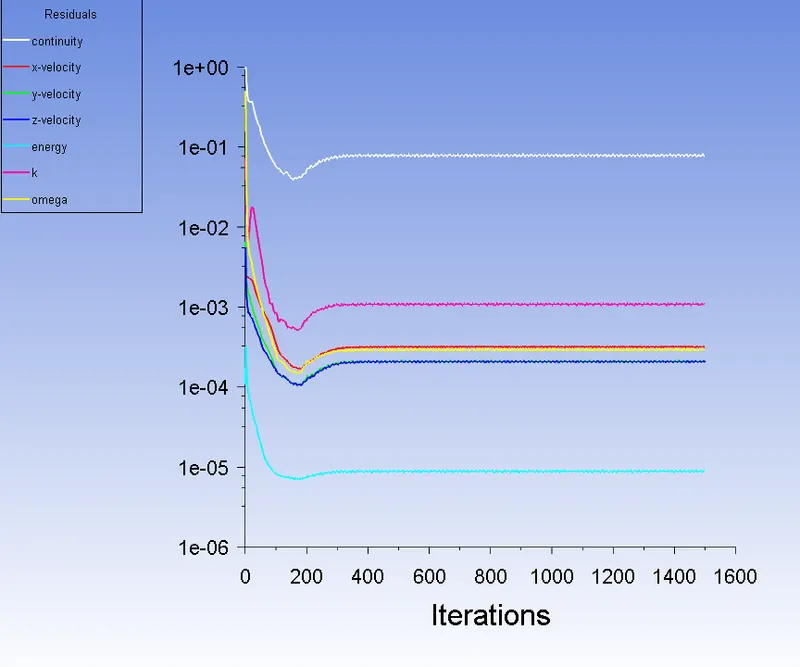
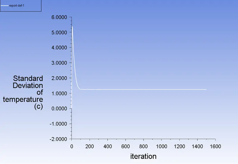
15. Now run program for till convergence criteria is satisfied.
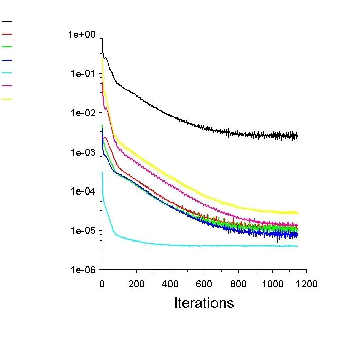
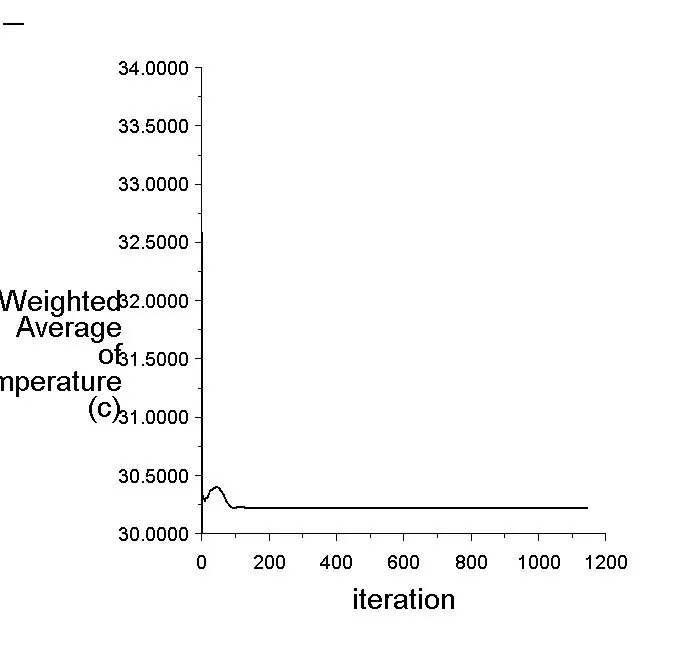
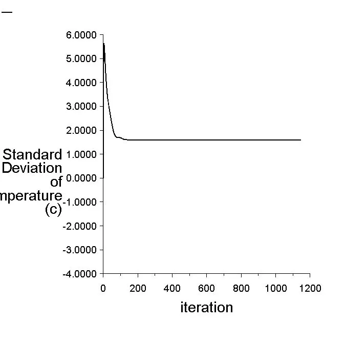
16. Repeat the same above stps for and change the turbulence to K-omega SST model and check for convergence.
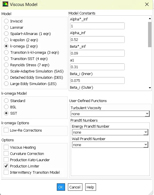
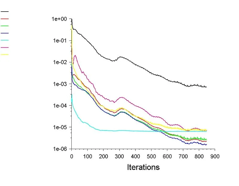
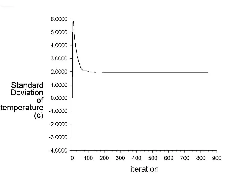
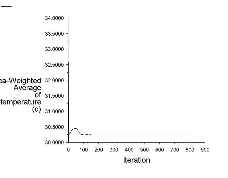
17. It was noted that 5mm mesh has lesser iterations for convergence in K-Omega SST than K-Realizable Epsilon.
18. So same steps as mentioned above was used for 3mm mesh and convergence is shown below.
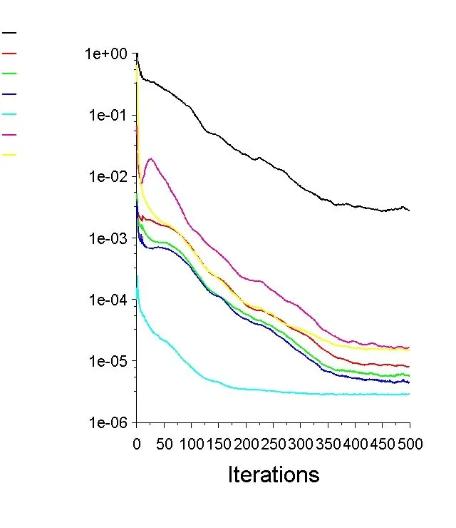
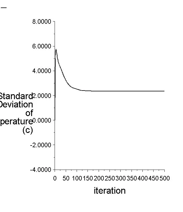
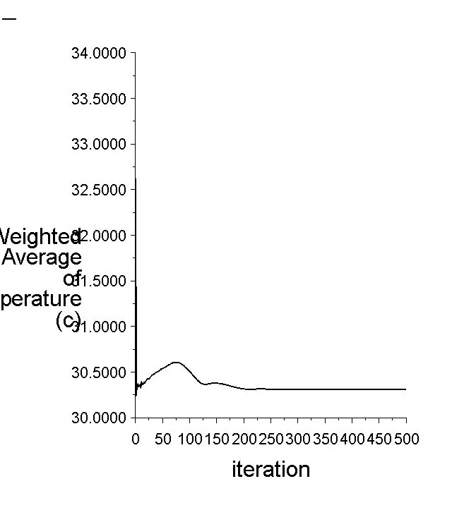
19. It was noted that 5mm mesh has lesser iterations for convergence in K-Omega SST than K-Realizable Epsilon.
20. So same steps as mentioned above was used for 1mm mesh and convergence is shown below.
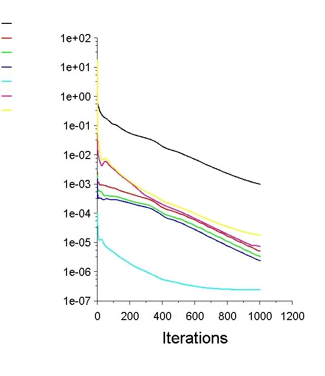
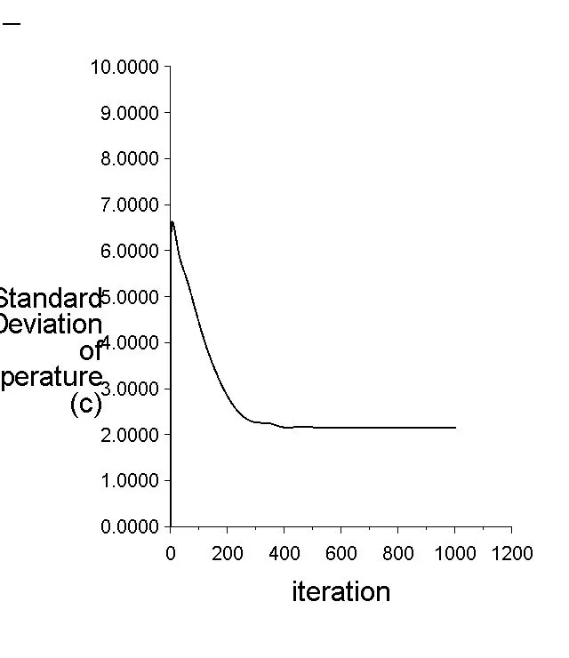
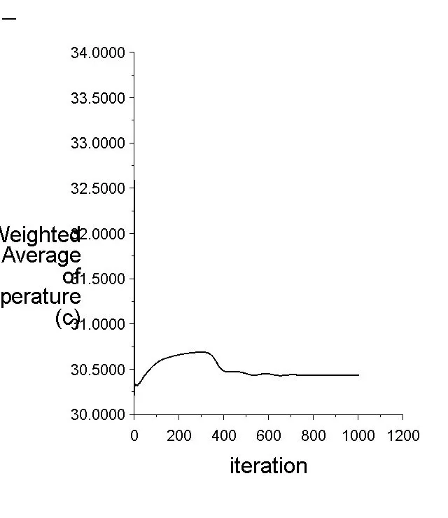
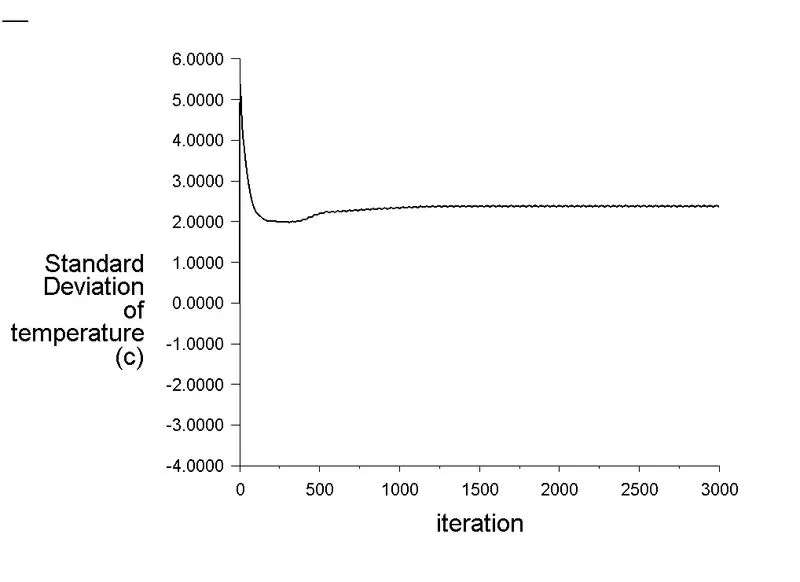
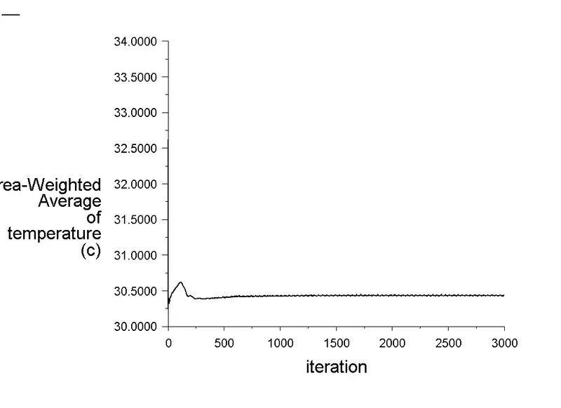
21. For longer tee, similar trend as seen in short tee was observed except for the increase in number of meshes and computation time.(5mm element length)
22. For longer tee, similar trend as seen in short tee was observed except for the increase in number of meshes and computation time.(3mm element length)

RESULT:

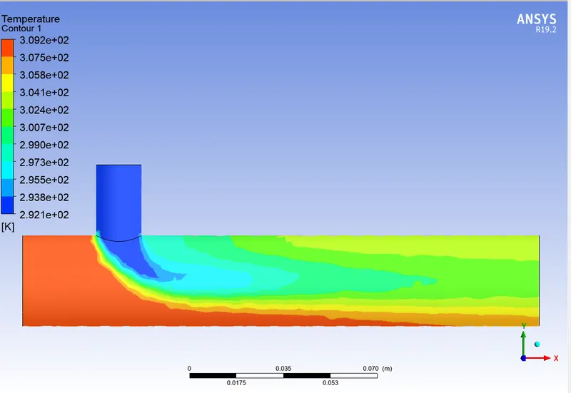
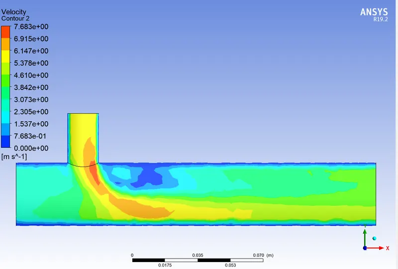
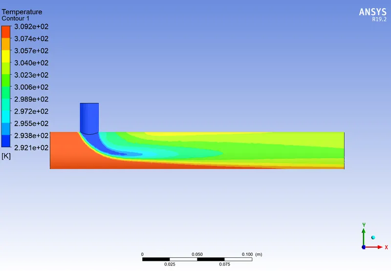
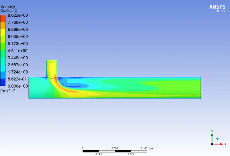
1. On post processing in CFD Post, select velocity and temperature contour is selected on a plane generated right at center of the mixing tee. (KEpsilon 5mm mesh-Short tee)
2. 
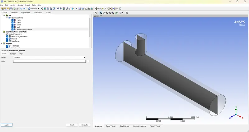
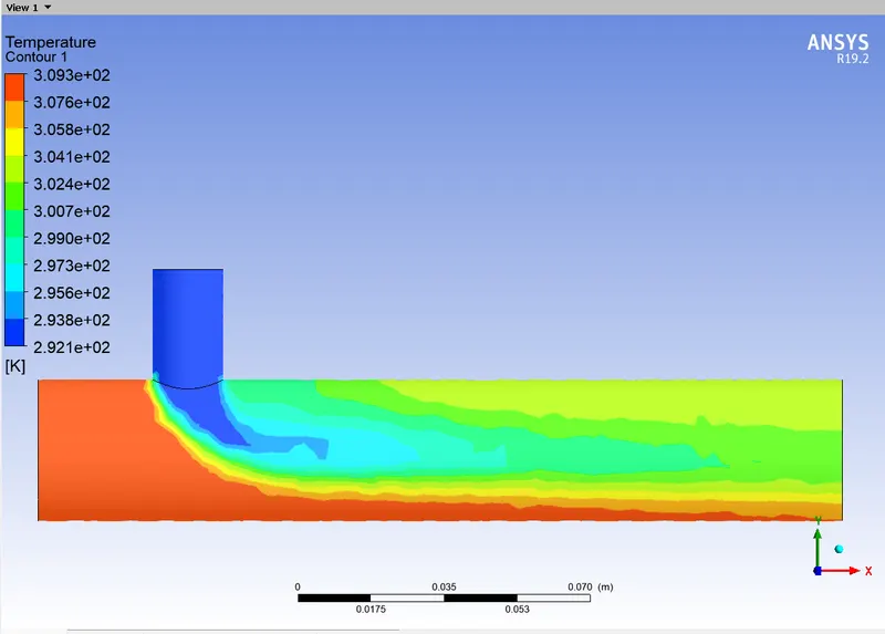
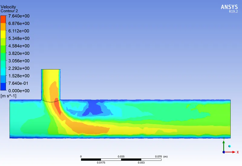
3. On post processing in CFD Post, select velocity and temperature contour is selected on a plane generated right at center of the mixing tee. (K-Omega SST 5mm mesh-Short tee)
4. It was noted that 5mm mesh has lesser iterations for convergence in K-Omega SST than K-Realizable Epsilon.
5. So same steps as mentioned above was used for 3mm mesh K-Omega SST and result in temperature and velocity contour is shown below.
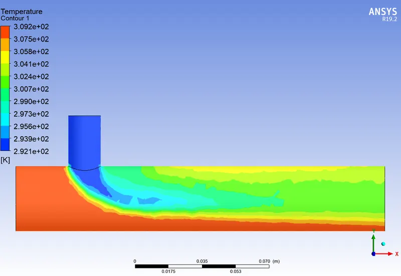
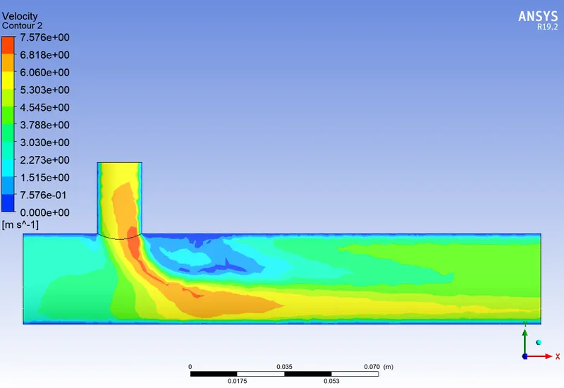
6. It was noted that 3mm mesh has lesser iterations for convergence in K-Omega SST.
7. So same steps as mentioned above was used for 3mm mesh K-Omega SST and result in temperature and velocity contour is shown below.
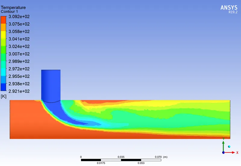
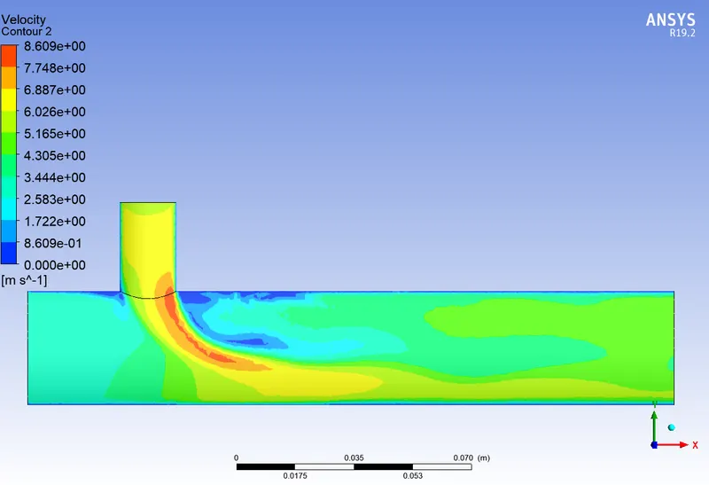
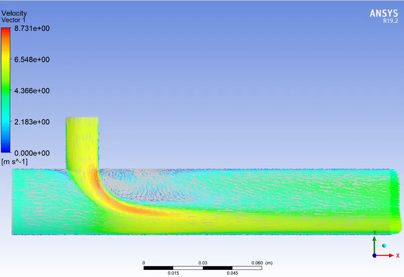
8. 5mm mesh length( longer tee )results.
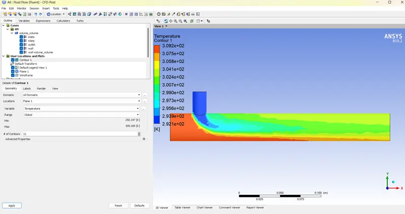
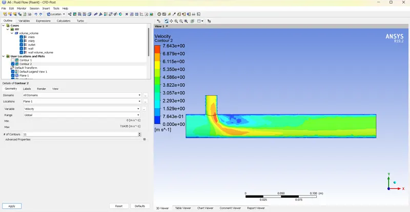
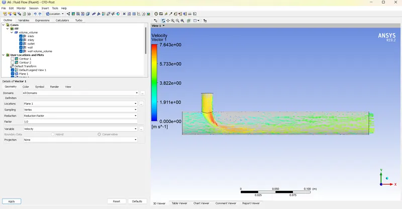
9. 3 mm mesh length(Longer tee)
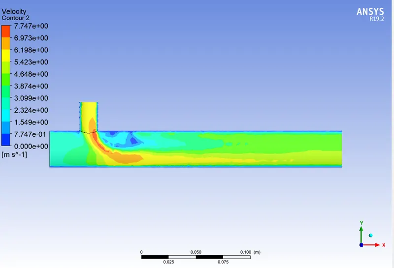
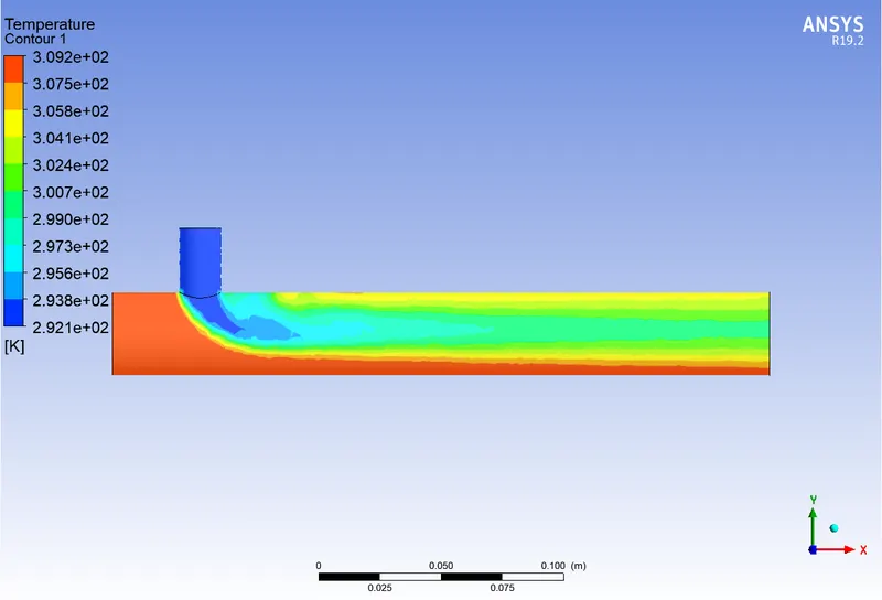
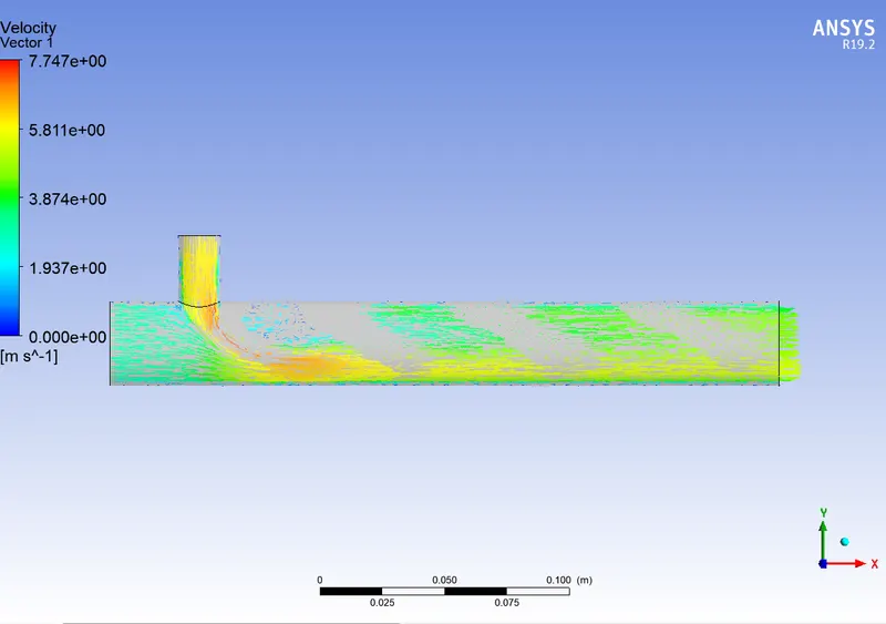
10. 1mm mesh length(longer tee)

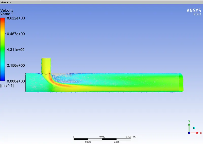
CONCLUSION:

1. It was noted that K-Omega SST model has lesser iterations to reach convergence than K-Realizable Epsilon for 5mm mesh.
2. So K-Omega SST model was selected for both 3mm and 5mm mesh.
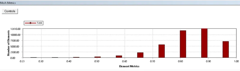
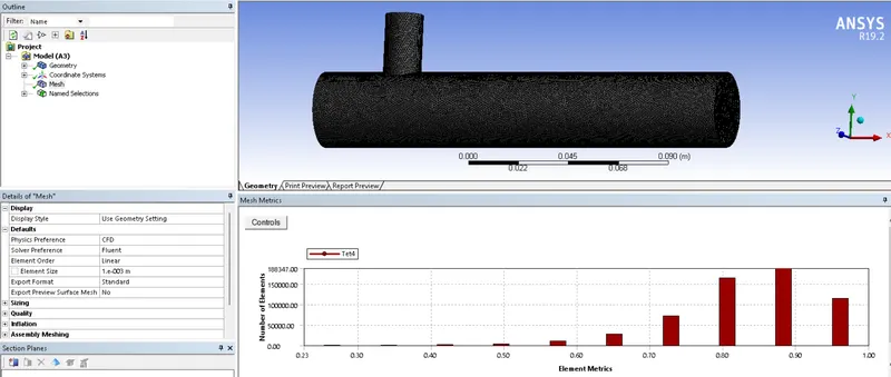
3. In all these caeses element metrics were found to have higher value than 5%. So Grid dependency test was only depending on convergence criteria. It was noted that Iterations to reach Convergence of 5mm mesh was best compared to both 3mm and 1 mm. But it was noted that results from tempretaure and velocity contour were not satisfactory. The time for iterations of 1mm mesh was too high to reach convergence but this opted to give best results. But 3mm mesh convergence time was totally staifiable and end results were far better than given by 5mm. so th best suited grid for further convergence for long tee was found to be 3mm.(Note: Grid dependency test is more valid on structured mesh).