Week 1- Mixing Tee
week 1 challenge:
aim:
- Case 1
- Short mixing tee with a hot inlet velocity of 3m/s.
- Momentum ratio of 2, 4.
- Case 2
- Long mixing tee with a hot inlet velocity of 3m/s.
- Momentum ratio of 2, 4.
tee joint.
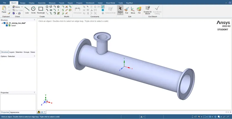
introduction:
A tee joint refers to the welded point of two metallic materials that are joined in the same plane at a 180° combined angle with a 90° angle on either side, forming the letter "T".
Welded tee joints are often prone to excess porosity, increased moisture entrapment, cracking and crevice corrosion due to the containment geometry generated by the degree at which it is formed.
A tee joint is a connection of two members approximately perpendicular to one another, forming two right angles similar to the letter T. This is a result of one member being connected between the two ends of the other. It differs from a corner joint consisting of a single right angle formed by two members each connected to the other at one end. Many types of members may be used to form tee joints including structural members of wood or metal, pipes or tubes made of concrete or plastic, and more.
There are several ways to form a tee joint. Materials may be adhesively bonded, and a variety of tee connectors are available to join certain types of members together. Members may also be connected with the use of fasteners such as nails or screws, or they may be notched to fit together like pieces of a puzzle.
theory::
ANSYS SOLUTION AND POSTPROCESSING
A typical ANSYS session, regardless of the discipline, involves the follow-
ing steps:
1. Model Generation
• SpQcify jobname (this step is optional but recommended).
• Enter Preprocessor,
• Define element types and options.
• Define real constant for the element types (if the element type(s)
require real constants).
• Define material properties.
• Create the model:.
- Build solid model (using either top-down or bottom-up approach).
- Define meshing controls.
• Create the mesh.
• Exit the Preprocessor,
2. Boundary/Initial Conditions and Solution
• Enter Solution Processor,
• Define analysis type and analysis options.
• Specify boundary/initial conditions:
• Degree of freedom constraints.
- Nodal force loads.
• Surface loads.
• Body loads.
• Inertia loads.
• Initial conditions (if the analysis type is transient).
• Save database (this step is not required but is recommended).
• Initiate solution.
• Exit the Solution Processor,
3. Review Results
• Enter the appropriate Postprocessor (General Postprocessor or Time
History Postprocessor),
• Display results.
solving and modelling:
- Step 1 : Pre-processing/Geometry Creation
- Launch Ansys workbench. Drag fluent into the work space.
- Open space claim. Import the geometry into space claim.
- As the given geometry is solid we need to perform volume extraction.
- Click on 'prepare' tab and select 'select edge' option. Select edges from inlets and outlets which will eliminate the solid part.
- Suppres the solid for physics. Close Space Claim.
- Update the project.
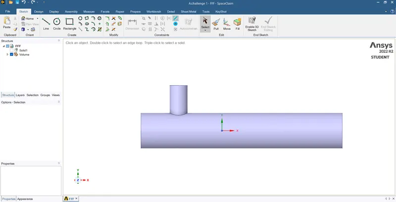
Figure of geometry after volume extraction.
- Step 2 : Mesh Generation
- Open mesh generator in ansys fluent.
- Selec the faces and name the each face accordingly as inlet (in x and y direction respectively), outlet and wall.
- Generate the default mesh.
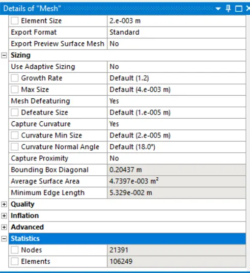
- Edit the element size to 0.002/2e-3m and update the mesh.
- Once the mesh is genertaed, close the mesh generator and update the project.
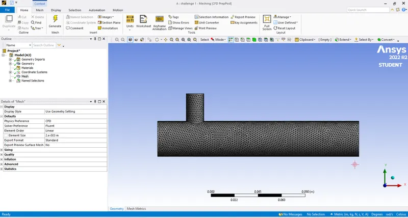
Figure of generated mesh for Short Tee joint.
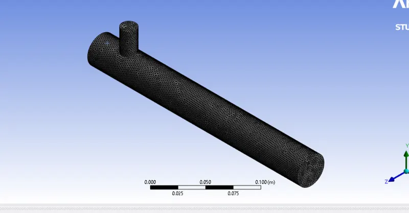
Figure of generated mesh for Long Tee joint.
- Step 3 : Solution Setup
- Open setup in fluent. The mesh and geometry will be generted. If it doesn't generate then go back to mesh generator and edit accordingly.
- Click on check mesh button. If the console doesn't show any warning then the mesh is fine.
- Click on Physics option and select pressure based solver, time as steady, velocity formulation as absolute and clickon Energy button as we need to solve the energy equation.
- In turbulence model select viscous k-epsilon realizable model.
- Click on solution and input the inlet data for each individual case. Outlet and wall conditions are already setup by fluent solver.
- Click on definitions and selected Area weighted Average and standard deviation for temperature at the outlet.
- Click on initialiaze button as the console will run calculation for 10 iterations.
- Click on Run calculation and set the number of iterations for 250 and hit the calculate button.
Inlet Conditions of the cases to be run :
- Hot inlet velocity = 3m/s, hot inlet temperature = 25 Celsius/298K; cold inlet velocity = 6m/s, cold inlet temperature = 10 Celsius/283K.
- Hot inlet velocity = 3m/s, hot inlet temperature = 25 Celsius/298K; cold inlet velocity = 12m/s, cold inlet temperature = 10 Celsius/283K.
Plots :
chapter1:
- Hot inlet velocity = 3m/s, hot inlet temperature = 25 Celsius/298K; cold inlet velocity = 6m/s, cold inlet temperature = 10 Celsius/283K.
- momentum of 2.
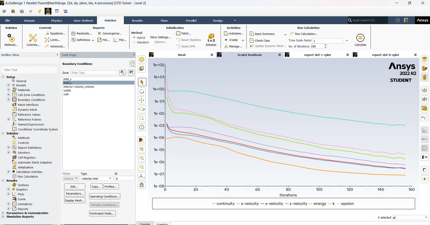
Figure shows plot of residuals versus number of iterations for Case 1.
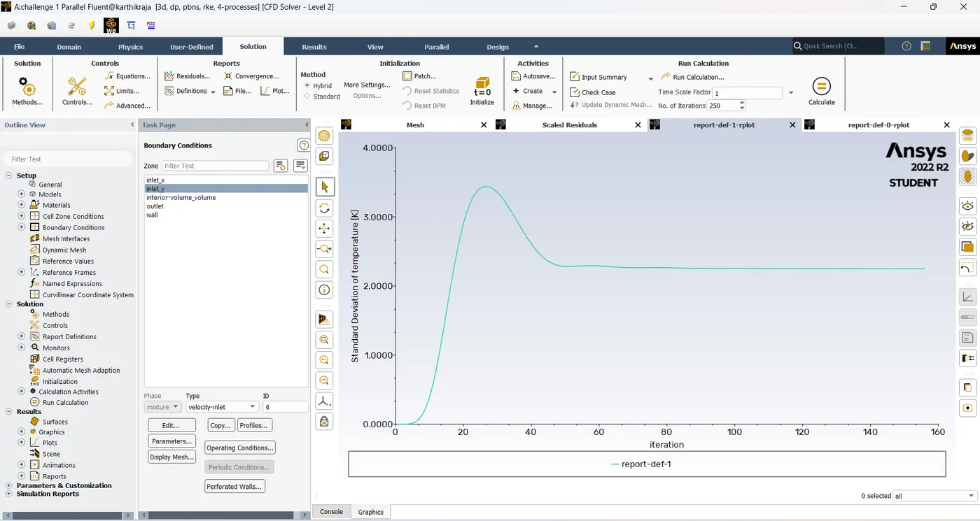
Figure shows plot of Standard Deviation of Temperature versus number of iterations for Case 1.
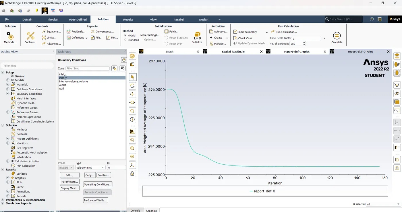
Figure shows plot of Area -Weighted Average of Temperature versus number of iterations for case 1
case2:
momentum of 4.
2.Hot inlet velocity = 3m/s, hot inlet temperature = 25 Celsius/298K; cold inlet velocity = 12m/s, cold inlet temperature = 10 Celsius/283K.
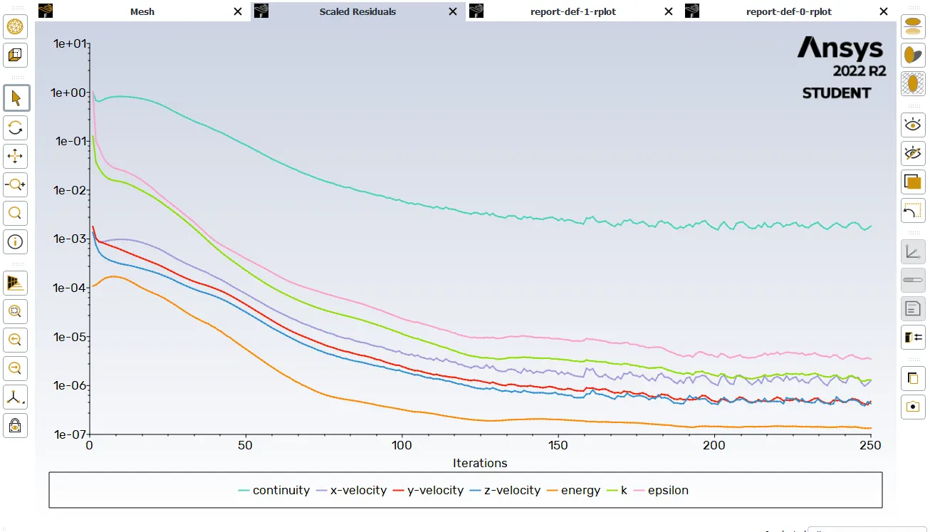
Figure shows plot of residuals versus number of iterations for Case 2.
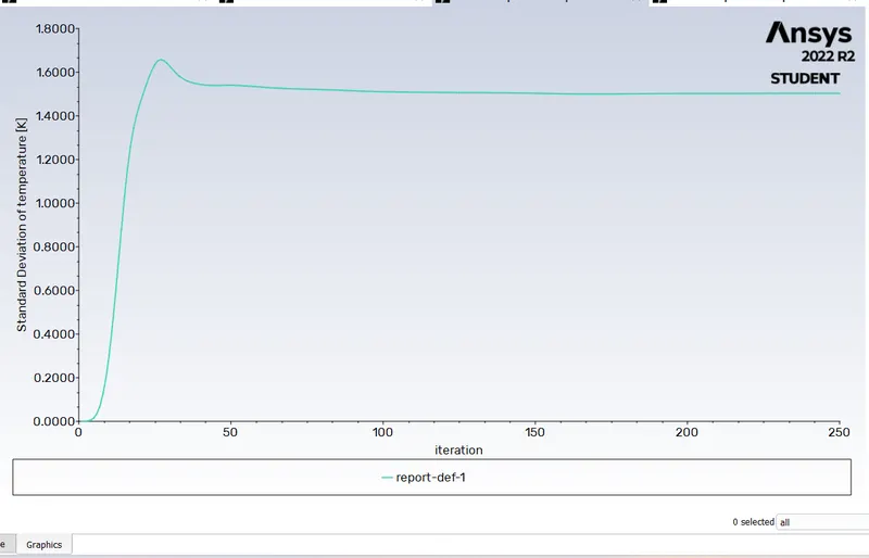
Figure shows plot of Standard Deviation of Temperature versus number of iterations for Case 2.
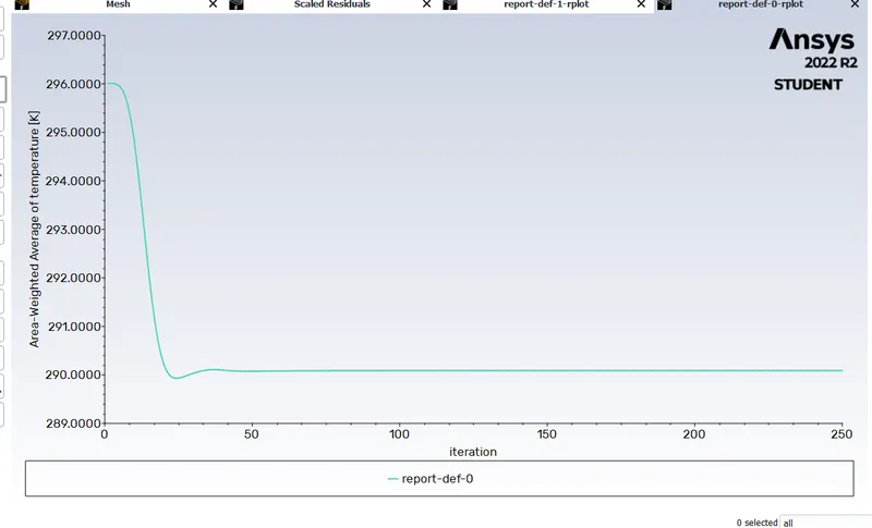
Figure shows plot of Area -Weighted Average of Temperature versus number of iterations for Case 2.
- Step 4 : Post-Processing
- Open Results viewer, a CFD post-processing tool, in Fluent.
- Increase the transperancy of the Tee section geometry by using the rendering button.
- Click on Insert option, then click on location and then select plane.
- In details of plane select the mode as variable and variable to be velocity or temperature.
- Set a user specified range of both quantities and click on apply.
- Capture the images to study the mixing of flows.
Plots
Case 1
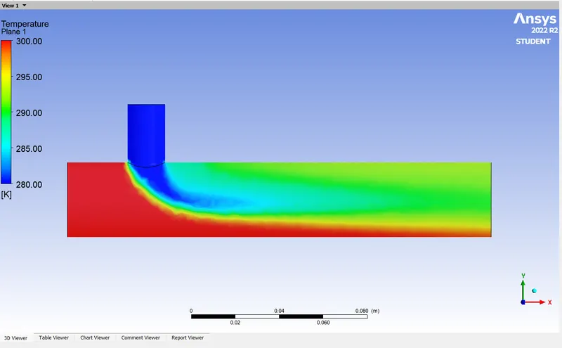
Figure shows the temperature distribution on a plane for Case 1.
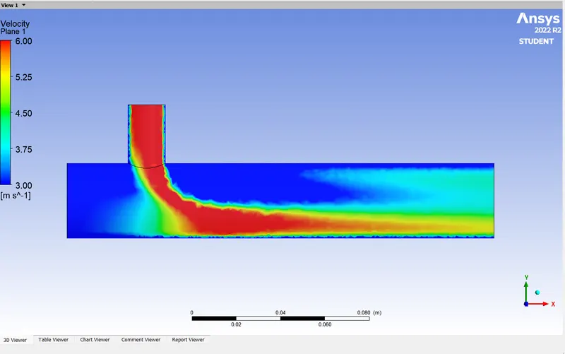
Figure shows the velocity distribution on a plane for Case 1.
Case 2
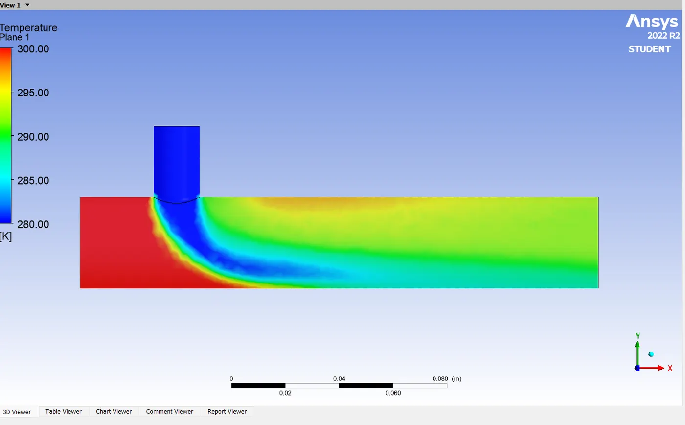
Figure shows the temperature distribution on a plane for Case 2.
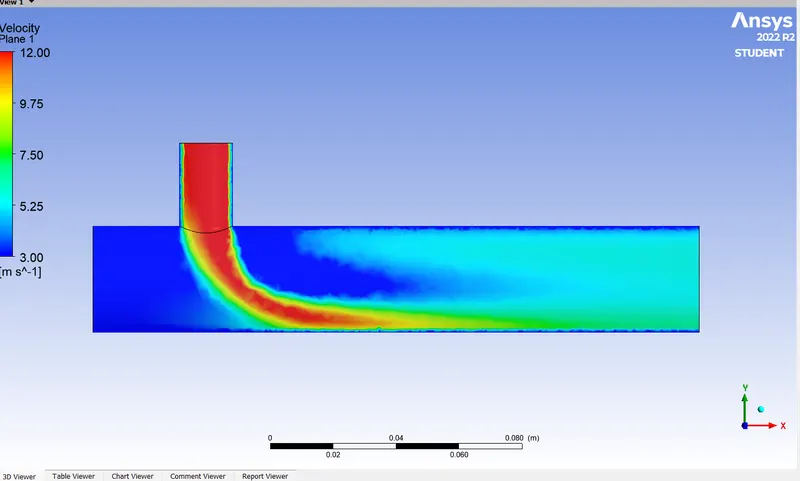
Figure shows the velocity distribution on a plane for Case .
- Results and Conclusion -
- for short tee joint.
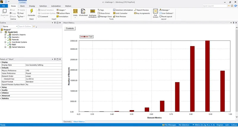
cell count:
no. of ieration:
chapter 2
this is same as the short tee . now let us see long tee:
Plots :
chapter2:
- Hot inlet velocity = 3m/s, hot inlet temperature = 25 Celsius/298K; cold inlet velocity = 6m/s, cold inlet temperature = 10 Celsius/283K.
- momentum of 2.
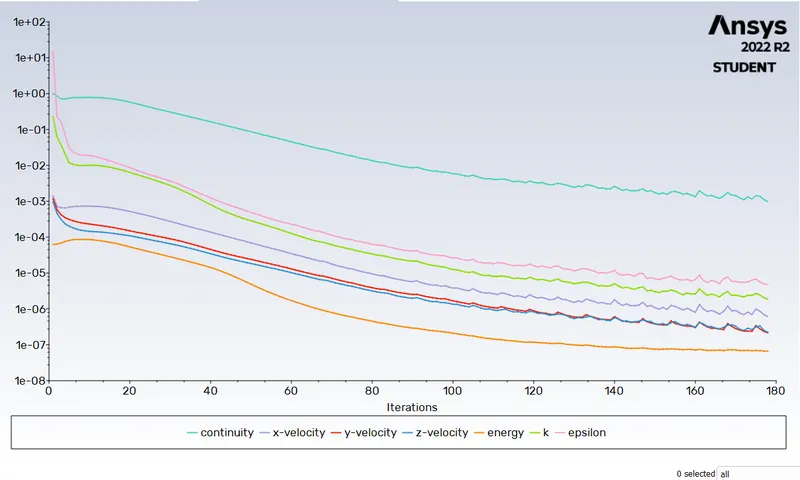
Figure shows plot of residuals versus number of iterations for Case 1.
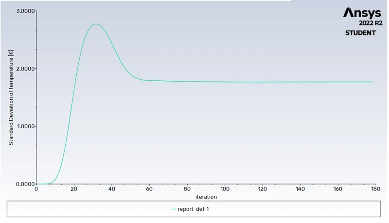
Figure shows plot of Standard Deviation of Temperature versus number of iterations for Case 1.
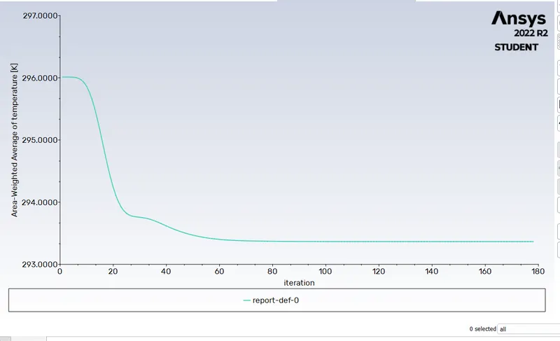
Figure shows plot of Area -Weighted Average of Temperature versus number of iterations for case 1
case2:
momentum of 4.
2.Hot inlet velocity = 3m/s, hot inlet temperature = 25 Celsius/298K; cold inlet velocity = 12m/s, cold inlet temperature = 10 Celsius/283K.
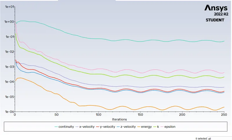
Figure shows plot of residuals versus number of iterations for Case 2.
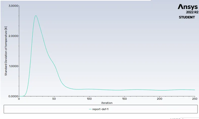
Figure shows plot of Standard Deviation of Temperature versus number of iterations for Case 2.
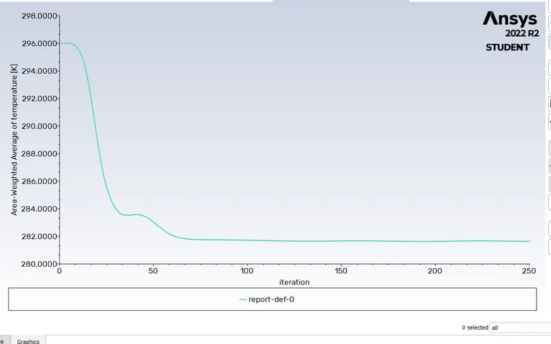
Figure shows plot of Area -Weighted Average of Temperature versus number of iterations for Case 2.
- Step 4 : Post-Processing
- Open Results viewer, a CFD post-processing tool, in Fluent.
- Increase the transperancy of the Tee section geometry by using the rendering button.
- Click on Insert option, then click on location and then select plane.
- In details of plane select the mode as variable and variable to be velocity or temperature.
- Set a user specified range of both quantities and click on apply.
- Capture the images to study the mixing of flows.
Plots
Case 1
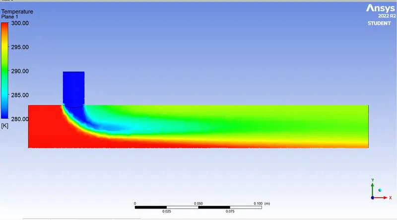
Figure shows the temperature distribution on a plane for Case 1.
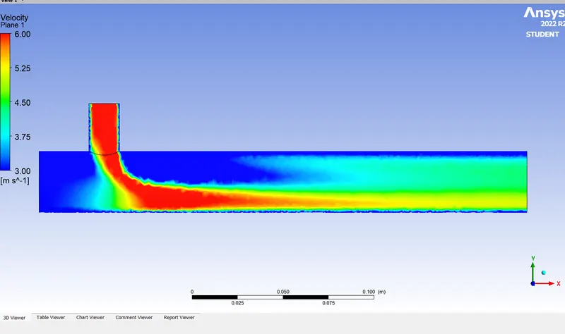
Figure shows the velocity distribution on a plane for Case 1.
Case 2
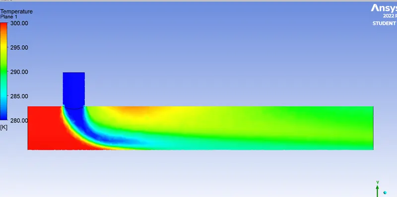
Figure shows the temperature distribution on a plane for Case 2.
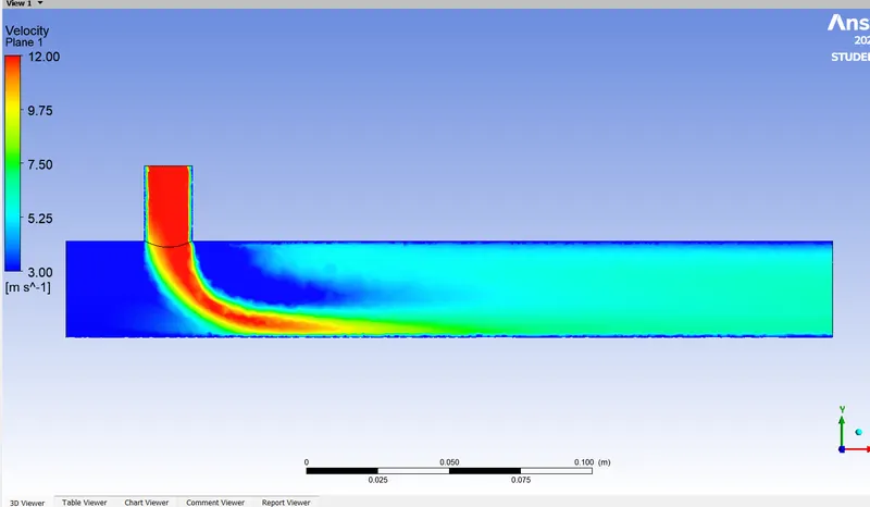
Figure shows the velocity distribution on a plane for Case .
- Results and Conclusion -
- for short tee joint.
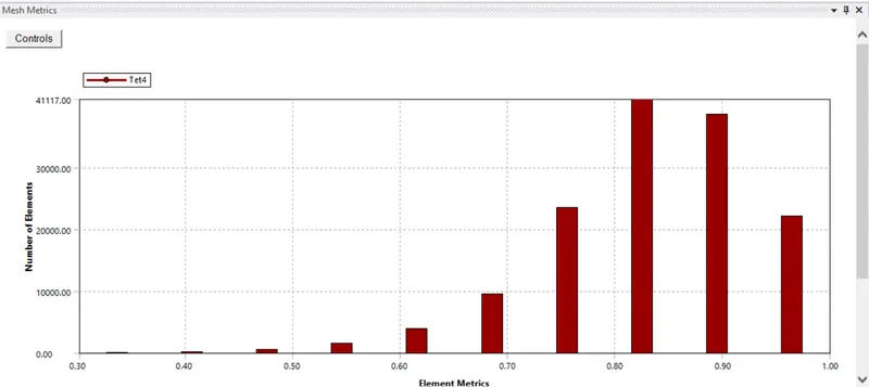
cell count:
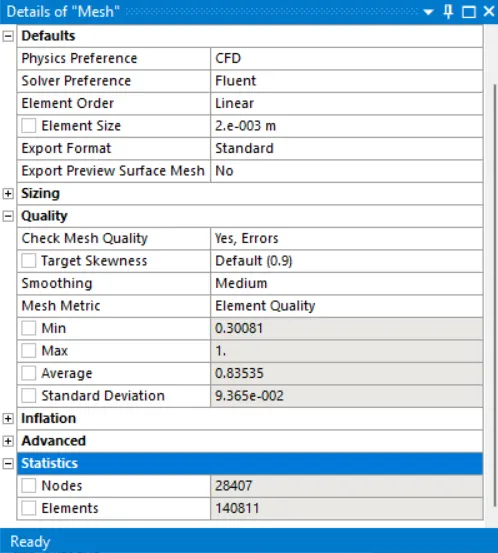
no. of ieration:
conclusion:
- In short Tee joint for both the cases, the velocity of cold inlet air plays a very big role. As we double the velocity we can see that the average outlet temperature has difference of 2.5 Celsius. Meaning we achieve better mixing of air with higher cold inlet velocity.
- In long Tee joint with velocity same as Case 1 for short tee, there isn't a significant change in average outlet temperature. Because of the increased length, the computational time and number of iterations to converge increased.
- We can concur that to achieve better mixing efficiency the velocity of inlet air plays major role. The length of the joint doesn't have any significant impact on thr mixing efficiency.
- From the plots we can see that the cold inlet air mixes well when the velocity is high. Finer loooking plots can be obtained with more fine mesh.
referance:
https://www.corrosionpedia.com/definition/6360/tee-joint
https://www.aboutmechanics.com/what-is-a-tee-joint.htm
------------------------------------------------------------------------------------------===thank you//===---------------------------------