Project 2 - Rankine cycle Simulator
aim:
to stimulate a rankine cycle and to plot the corresponding t-s and h-s diagram using matlab.
objective:
calculate the state of the rankine cycles.
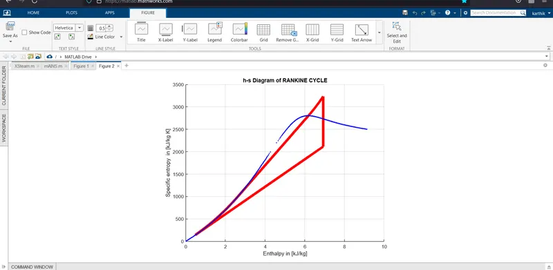
plotting the t-s and h-s graph.
given:
inpu value:
turbine input temperature=400 degree celcisus.
turbine input pressure=30 bars.
turbine output pressure=0.05 bars.
required output':
network output.
backwork ratio.
introduction:
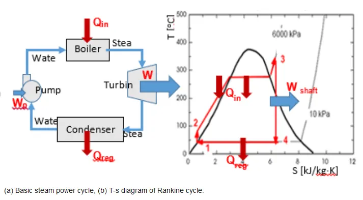
rankine cycle converts thermal energy into mechancial energy.
it consist of four process which are:
1. 1-2 adiabatic compression in pump
2. 2-3 constant pressure heat addition in boiler
3. 3-4 adiabatic expansion in turbine
4. 4-1 constant pressure heat rejection in condenser
rankine cycle process:
general procedure to calculate the thermal state:
first, all the required variable parameter were found out to calculate.
then using the xsteam table function all the parameters are sorted out.
then usual calculation and plot t-s and h-s diagram.
clear all
close all
clc

%printing heading
fprintf('rankine cycle:\n\n')
fprintf('1-2 adiabatic compression process in pump\n')
fprintf('2-3 constant pressure heat addition in boiler\n')
fprintf('3-4 adiabatic expansion in turbine\n')
fprintf('4-1 constant heat rejection in condensor\n')

% input from the user:
p1=input('\nenter the initial pressure of turbine:\n')
t1=input('enter the initial temperatur of turbine:')
p2=input('enter the final pressure of turbine:\n')

% State variable at state point 1:
h1 = XSteam('h_pT',p1,t1);
s1 = XSteam('s_pT',p1,t1);
v1 = XSteam('v_pT',p1,t1);

% at state point 2:
s2 = s1;
h2 = XSteam('h_px',p2,XSteam('x_ps',p2,s2));
t2 = XSteam('T_ps',p2,s2);
v2 = XSteam('v_ps',p2,s2);

%at state point 3:
p3 = p2;
t3 = XSteam('Tsat_p',p3);
h3 = XSteam('hL_p',p3);
s3 = XSteam('sL_p',p3);
v3 = XSteam('vL_p',p3);

%at state point 4:
s4 = s3;
p4 = p1;
h4 = XSteam('h_ps',p4,s4);
t4 = XSteam('T_ps',p4,s4);
v4 = XSteam('v_ps',p4,s4);

t_range = linspace(0,374.15,500);

%plotting the t-s diagram;
figure(1)

%Ploting Graph for value of Rankine cycle in t-s.
figure(1)
hold on
plot([s1 s2],[t1 t2],'color','r','LineWidth',5);
plot([s2 s3],[t2 t3],'color','r','linewidth',5);
plot([s3 s4],[t3 t4],'color','r','linewidth',5);
Trange = linspace(t4,t1,500);
for i = 1:length(Trange)
    s_range(i) = XSteam('s_pT',p1,Trange(i));
    h_range23(i) = XSteam('h_ps',p1,s_range(i));
    h_range41(i) = XSteam('h_ps',p2,s_range(i));
end
plot(s_range,Trange,'color','r');

%plotting the cycle:
for i = 1:length(t_range)
    plot(XSteam('sL_t',t_range(i)),t_range(i),'.','color','b')
    plot(XSteam('sV_t',t_range(i)),t_range(i),'.','color','b')
end

% Ploting Graph for value of Rankine cycle in h-s.
figure(2)
hold on
plot([s1 s2],[h1 h2],'color','r','linewidth',5);
plot(s_range,h_range23,'color','r','linewidth',5);
plot([s3 s4],[h3 h4],'color','r','linewidth',5);
plot(s_range,h_range41,'color','r','linewidth',5);

for i = 1:length(t_range)
    plot(XSteam('sL_t',t_range(i)),XSteam('hL_t',t_range(i)),'.','color','b')
    plot(XSteam('sV_t',t_range(i)),XSteam('hV_t',t_range(i)),'.','color','b')
end

% Ploting Diagram for All state points forRankine cycle in t-s:
figure(1)
hold on
plot(s1,t1)
plot(s2,t2)
plot(s3,t3)
plot(s4,t4)
grid on
title('T-s Diagram of RANKINE CYCLE')
xlabel('Temperature in [degree C]')
ylabel('Specific entropy  in [kJ/kg K]')

%Ploting Diagram for All state points for Rankine cycle in h-s:
figure(2)
hold on
plot(s1,h1)
plot(s2,h2)
plot(s3,h3)
plot(s4,h4)
grid on
title('h-s Diagram of RANKINE CYCLE')
xlabel('Enthalpy in [kJ/kg]')
ylabel('Specific entropy  in [kJ/kg K]')

% calculations

% Turbine Work
Wt = h1-h2;

% Pump Work
Wp = h4-h3;

% Heat Addition
Qin = h1-h4;

% Heat Rejection
Qout = h2-h3;

% Net Work
Wnet = Wt-Wp;

% Efficiency
Ntherm = (Wnet/Qin)*100;

% Specific steam consumption
SSC = 3600/Wnet;

% Back Work Ratio
BWR = Wp/Wt;

% output diplay:

fprintf('results\n\n')
fprintf('at state point 1\n')
fprintf('p1 is:%.3f bar\n',p1)
fprintf('T1 is:%.3f degree celcius\n',t1)
fprintf('H1 is:%3.f kj/kg\n',h1)
fprintf('s1 is:%.3f kj/kg.k\n\n',s1)

fprintf('at state point 2\n')
fprintf('p2 is:%.3f bars\n',p2)
fprintf('T2 is:%.3f degree celcius\n',t2)
fprintf('H2 is:%.3f kj/kg\n',h2)
fprintf('s2 is:%.3f kj/kg.k\n\n',s2)

fprintf('at state point 3\n')
fprintf('p3 is:%.3f bars\n',p3)
fprintf('T3 is:%.3f degree celcius\n',t3)
fprintf('H3 is:%.3f kj/kg\n',h3)
fprintf('s3 is:%.3f kj/kg.k\n\n',s3)

fprintf('at state point 4\n')
fprintf('p4 is:%.3f bars\n',p4)
fprintf('T4 is:%.3f degree celcius\n',t4)
fprintf('H4 is:%.3f kj/kg\n',h4)
fprintf('s4 is:%.3f kj/kg.k\n\n',s4)

fprintf('wt is:%.3f kj/kg\n',Wt)
fprintf('wp is:%.3f kj/kg\n',Wp)
fprintf('wnet is: %.3f kj/kg\n',Wnet)
fprintf('ntherm is:%.3f percent\n',Ntherm)
fprintf('s s c is:%.3f Kg/KWh',SSC)
procedure for rankine cycle:
first we have to open the matlab, and create a new script.
write close all, clear all, clc to close the previous work.then start to write the code.
firstly we have to print the introduction for our code using fprintf code. then we have to get the input from the end user such as temperture, pressure of turbine at intial condition.
now with the help of the thermodynamic formula calculate the all the state temperature, pressure, enthalpy, entropy and volume.
then find the work done in pump, work done in turbine, heat addition, heat rejection and specific steam consumption.
now plot the t-s and h-s diagram for the given user value. and compare with the saturation curve.
then display all the state values by using fprintf command in matlab.
output:
result in command window
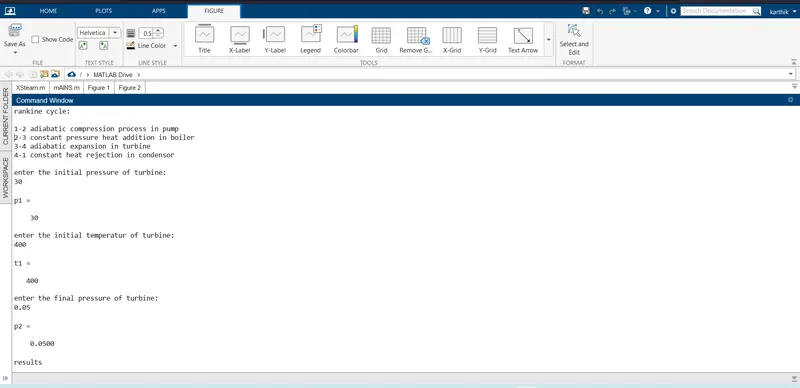
page 1 of 2
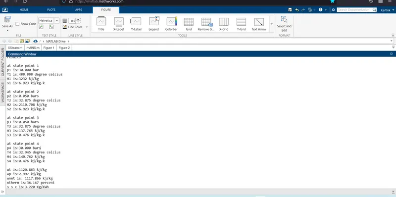
page 2 of 2
rankine cycle t-s and h-s diagram:
temperature vs entropy:
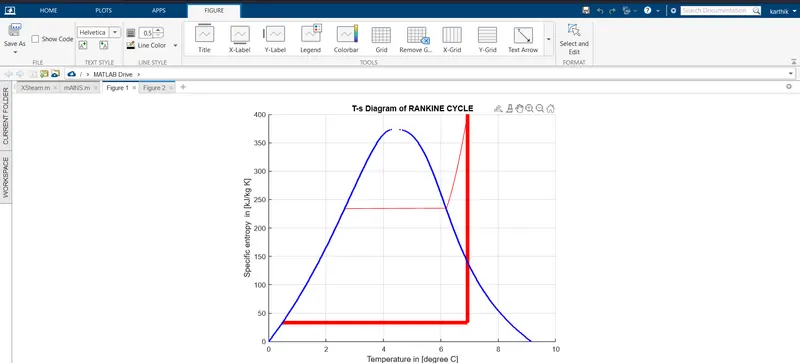
enthalpy vs entropy:
conclusion :
the t-s and h-s diagram is ploted by using matlab and the results of the states are shown in the above.