Week 1- Mixing Tee
AIM : MIXING TEE CFD SIMULATIONS OF THE TEMP AND VELOCITY AT DIFFRENT PORTIONS OF MIXING TEE.
PROBLEM STATEMENT:
For this challenge, we have created two versions of the mixing tee. One of them is longer than the other.
Your job is to set up steady-state simulations to compare the mixing effectiveness when hot inlet temperature is 360C & the Cold inlet is at 190C.
Use the k-epsilon and k-omega SST model for the first case and based on your judgment use the more suitable model for further cases. Giving the reason for choosing a suitable model is compulsory.
- Case 1
- Short mixing tee with a hot inlet velocity of 3m/s.
- Momentum ratio of 2, 4.
- Case 2
- Long mixing tee with a hot inlet velocity of 3m/s.
- Momentum ratio of 2, 4.
Momentum ratio = velocity at cold inlet / velocity at hot inlet
In a table, compare the following values from the 2 cases.
- Cell count
- Average outlet temperature
- Number of iterations for convergence.
INTRODUCTION THEORY:
Tee flow it calls as tee because it splits the flow and angle betwwen them is 90.
This type of flow are widely used in the practical applications such as in air conditioning where the cold air having low temperature and having some velocity is mixed with the warm atmospheric air having high temperature to reduce the atmospheric air temperature to some extent which is comfortable for the human body.
Solving and modelling approach:
To perform the above in the ANSYS there are mainly 3 steps to perform the simulations in the ansys fluent.
1) Pre processing : This step involve prepping up the geometry for the required simulation.
> Importing the geometry , extracting the fluid volume etc. are some of the steps in the procedure.
> descretizing the domain is sometimes regarding as preprocessing step.
> Ansys SPACECLAIM and WORKBENCH MESHER are the tools used here.
2) Solving: This step consist the following.
> initial conditions
> boundary conditions : boundary conditions are specified to let the solver know that a particular region of space is to have a particular value.This value will persist throughout the simulations.They are dependent on space not time.Since the solver will solve the set of diffrential equations, boundary conditions help us get exact solution of these equations.
> Material properties
> Turbulence models
3) Post processing :
> Used to analyse the results after solving.
> You can get contor plots, line plots, charts etc and export the data.
Procedure to simulate the flow through an mixing tee:
STEP 1:
> Create a computational model using ANSYS SPACE CLAIM.
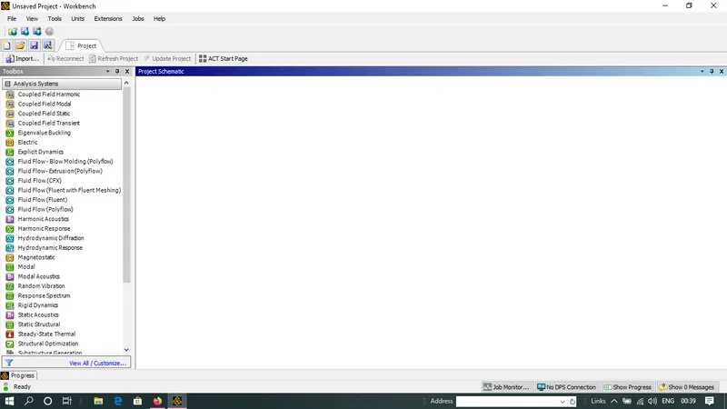
ANSYS WORKBENCH > Drag fluid flow(fluent) from analysis system > Drop it on Project schematic. > dole click on geometry at the left corner a msg appear that is starting spaceclaim > file > open > select mixing tee short geometry > open > extract fluid vloume > prepare > volume extraction > select dge option > select edges > click on green colour tick mark > structure > hide solid component > wet volume.
To make sure solid model is not used for simulation.
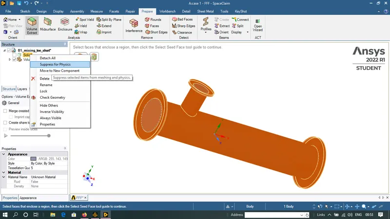
Right click on solid > supress for physics .
Close the window things will automatically get saved.
> Spaceclaim is a CAD cleanup software that can used for the preparation of CAD models for the simulation setup for CFD.
>
K-epsilon turbulent model:
The K-epsilon model is one of the most common turbulence models, although it just doesn't perform well in cases of large adverse pressure gradients. It is a two equation model, that means, it includes two extra transport equations to represent the turbulent properties of the flow. This allows a two equation model to account for history effects like convection and diffusion of turbulent energy.
The first transported variable is turbulent kinetic energy, . The second transported variable in this case is the turbulent dissipation, . It is the variable that determines the scale of the turbulence, whereas the first variable, , determines the energy in the turbulence.
The K-epsilon model has been shown to be useful for free-shear layer flows with relatively small pressure gradients. Similarly, for wall-bounded and internal flows, the model gives good results only in cases where mean pressure gradients are small; accuracy has been shown experimentally to be reduced for flows containing large adverse pressure gradients. One might infer then, that the K-epsilon model would be an inappropriate choice for problems such as inlets and compressors.
K-omega turbulent model:
The k-omega () turbulence model is one of the most commonly used models to capture the effect of turbulent flow conditions. It belongs to the Reynolds-averaged Navier-Stokes (RANS) family of turbulence models where all the effects of turbulence are modeled.
It is a two-equation model. That means in addition to the conservation equations, it solves two transport equations (PDEs), which account for the history effects like convection and diffusion of turbulent energy. The two transported variables are turbulent kinetic energy (), which determines the energy in turbulence, and specific turbulent dissipation rate (), which determines the rate of dissipation per unit turbulent kinetic energy. is also referred to as the scale of turbulence.
Case Studies:
There are mainly two cases that we have to perform the simulation one for the shorter length T-pipe and one for the longer length T-pipe. But we also have to run the simulations for different momentum ratios and different turbulent models so in total we have to run 5 cases.
| Cases | Momentum Ratios | Length | Turbulent Model |
| Case 1 | 2 | Short | K-epsilon |
| Case 2 | 2 | Short | K-omega |
| Case 3 | 4 | Short | - |
| Case 4 | 2 | Long | - |
| Case 5 | 4 | Long | - |
> We first have to decide which turbulence model is more preferable than the other.
Case Set-up:
In the case set-up procedure we will be preparing our geometry ready for the simulation.
> Open the project schematic window in Ansys and open Fluid Flow(Fluent).
1. Geometry import:
We first have to import the gemoetry into the Ansys Spaceclaim.
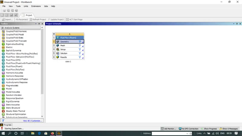
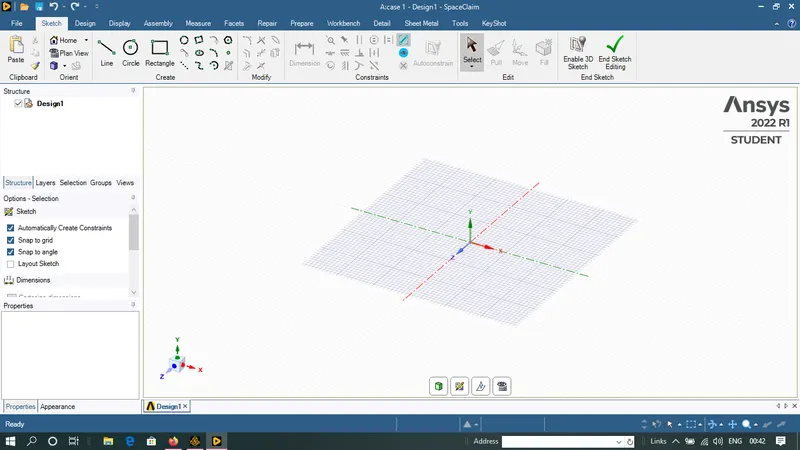
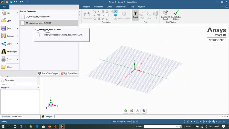
Now we have to extract the geometry suitable for the simulation where the fluid actually flows.
Prepare > volume extract > select edge > selecting the three edges without pressing the ctr key. > click on the tick mark.
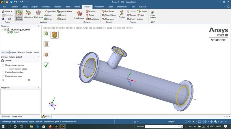
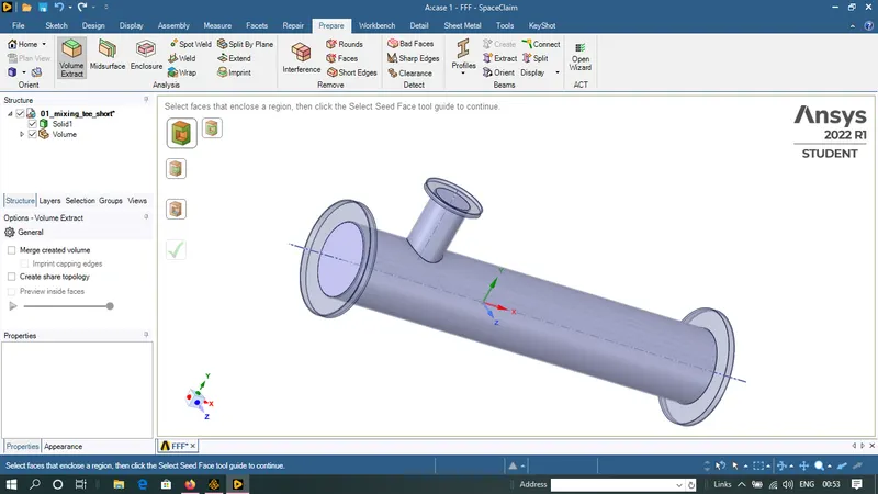
untick the solid 1 > right click on solid 1 > select suppress for physics.
By using the suppress for physics the solid portion of the body will not be participated for the further iterations.
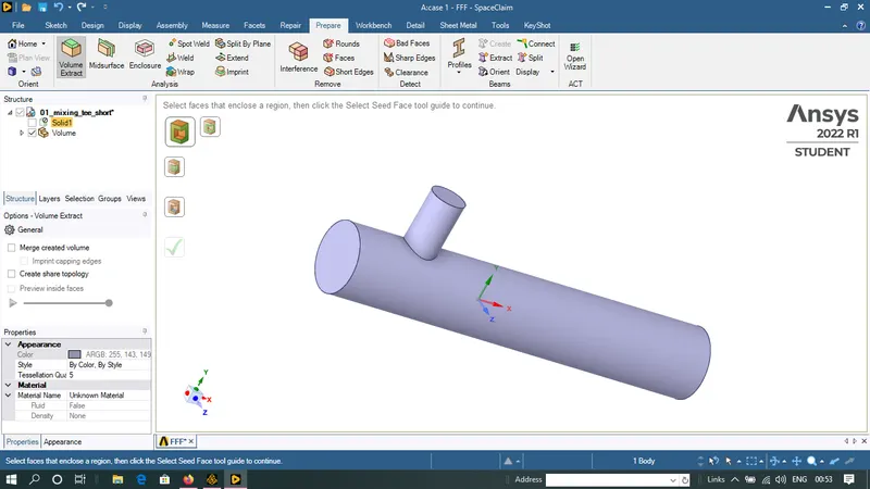
> Below is the final body throgh which fluid will flow and used for the simulation.
STEP 2:
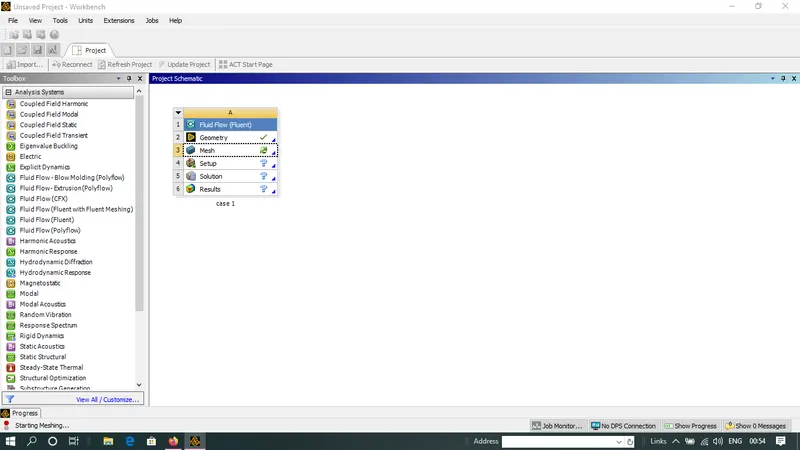
> Double click on mesh.
Project schematic > Mesh > double click.
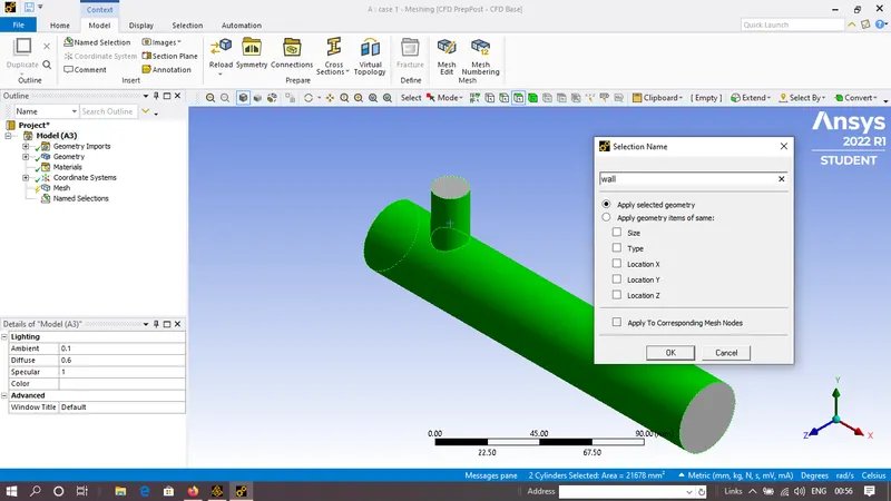
> Name the boundaries where the mesh has to be performed.
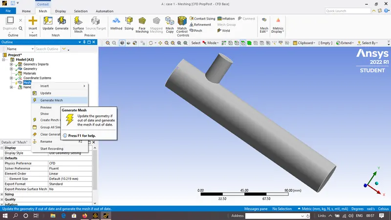
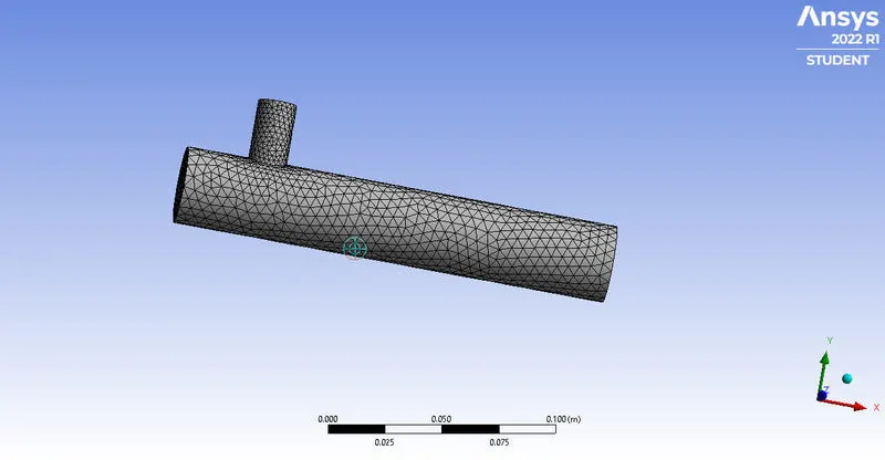
Project schematic > mesh > ctr f for face selection > click on face > press N key for name selection > enter name for the diffrent faces > Project (at left side) > mesh > details of mesh > sizing > Most of the properties are set because Fluent has uses a bounding box > Right click on mesh > click on generate > mesh will be generated on the fluid body.
> Bounding box is the smallest box where the whole geometry can be fit inside.So based upon this box Ansys fluent will automatically create the mesh element.
> To view the sctional view of the plane follow the layout.
Put the geometry in y direction > New section plane > click and drag to create a line.
> Perform the name selection for the diifrent parts of the body.
Right click on mesh and generate mesh with element size of 5mm.
STEP 3:
Details of mesh > Quality > select mesh metric as ELement quality .
> At x-axis we have element matrices that is element quality and along y-axis we have number of elements.
> Here the minimum quality is 40% and maximum quality is 100%.
> In order to measure the Quality we should know finite volume method, interpolation schemes, Aspect ratio, skewness, orthogonallity.
> Element Quality should not be less then 5% in this case it is 0.4 i,e, 40%.
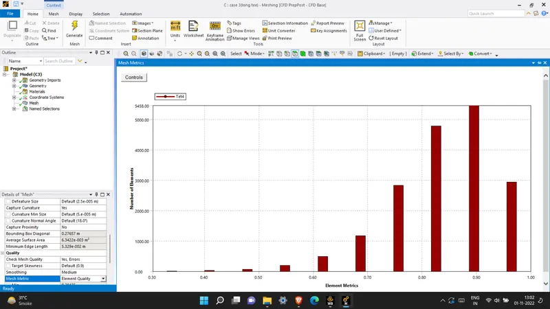
Note: As we are going to choose the element size of 5mm in every case, the mesh and the mesh quality plot is going to be the same for every case.
STEP 4:
Move to ansys fluent and set the diffrent conditions such as
> initial conditions
>boundary conditions
>Numerics
In this case employ the steady state solver in a pseudo transient mode .
For the Turbulence model use K-epsilon method.
Define convergence criteria.
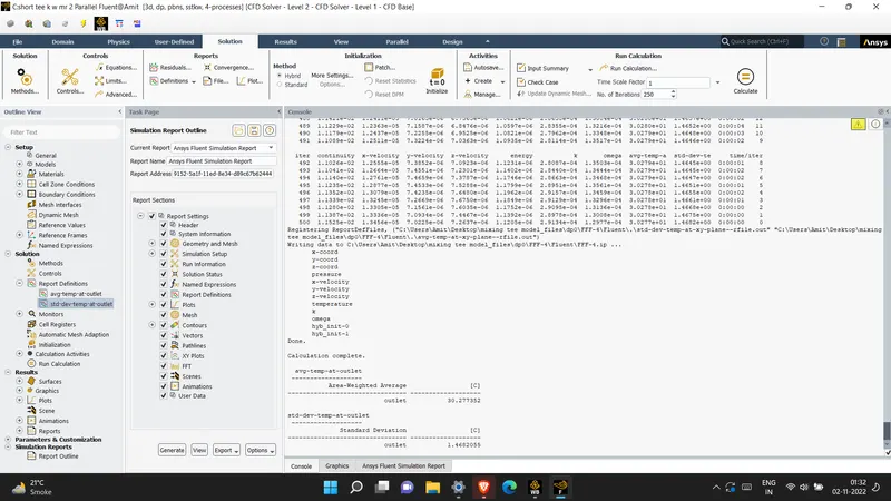
> CONSOLE is the place where the important information regarding the geometry,simulation shown up.
Case 1:
Parameters:
| Length | Short |
| Momentum Ratio | 2 |
| Hot air velocity with temperarure (oC) | 3m/s ; 36 |
| Cold Air velocity with temperature(oC) | 6m/s ; 19 |
| Element Size | 5mm |
| Number of Elements | 14250 |
| Turbulence Model | K-epsilon (standard) |
> To perform the simulation follow the layout as mentioned below.
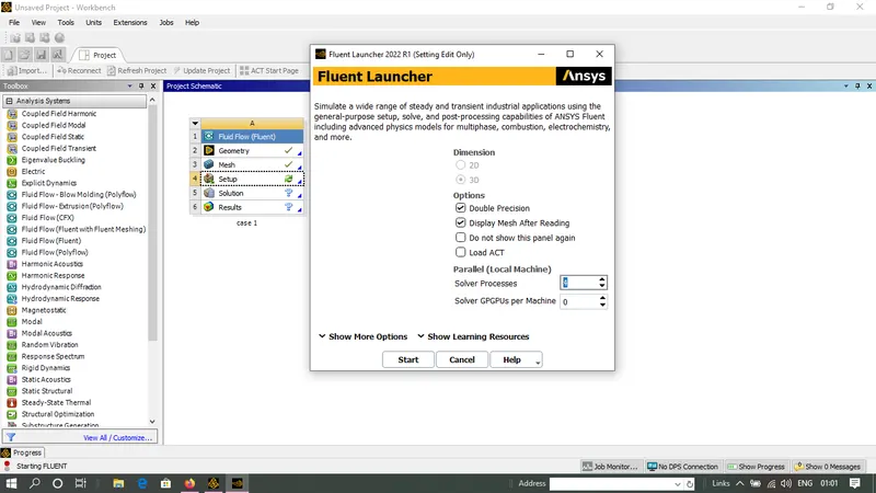
Project schematic > Fluid fluent(fluent) > setup > double click > Ansys fluent will launch > select double precision > proceesor as 4.
sometimes ansys fluent will not run the mesh object in its graphics window for such cases close the window and again open the setup by follwing the same layout as mentioned above.
>
Check the mesh quality by following the layout.
Setting up domain > click on check key. > console > at bottom side of display there is text present which is "checking mesh done".
if there is no warning message that means mesh is ok.
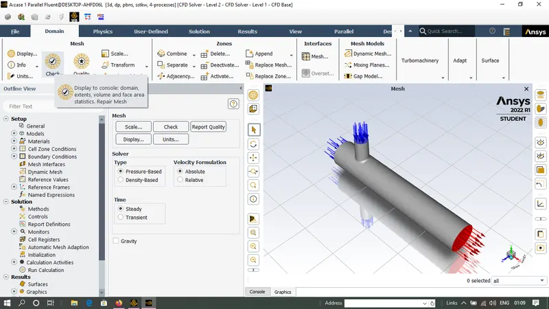
> Setting up physics > time > steady state solver > type > Pressure based > velocity formation > absolute > as we are interested to solve for temp which reqiures Energy equations >
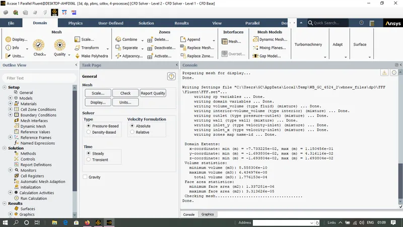
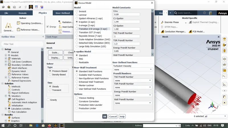
Energy > viscous Model > Model > K-epsilon > k-epsilon mode > Realizable > Near wall treatment > standard walll functions > ok > Materials > air > zones > cell zones > select volume region > boundaries > inlet x > type > velocity inlet > edit > momentum > velocity magnitude as 3m/s > thermal > temperature as 36 > inlet y > edit > momentum > velocity magnitude as 6m/s > Thermal > temperature as 19.
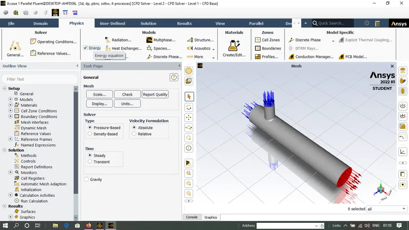
> select the Turbulence model as k-epsilon model.
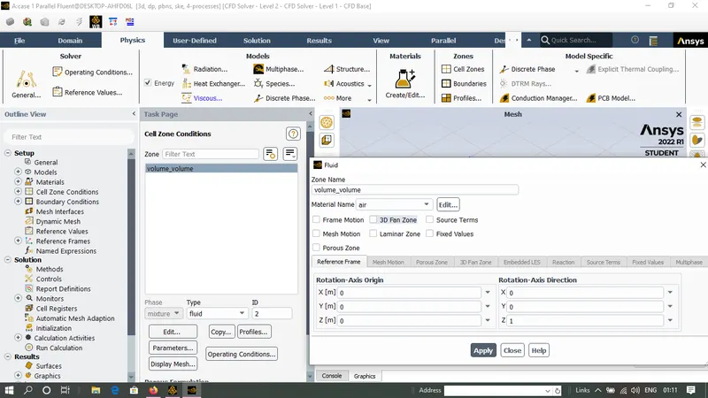
> check the cell zones condition.
> Select the boundary conditions for the inlet x and inlet y .
> For inlet x select velocity as 3m/s and temperature as 36oC.
> For inlet y cold fluid velocity as 6m/s and temperature as 19oC.
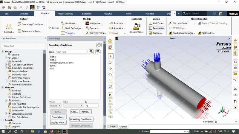
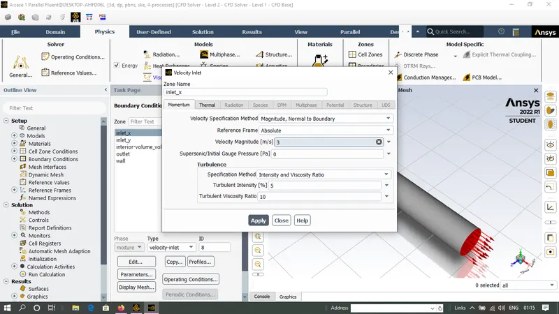
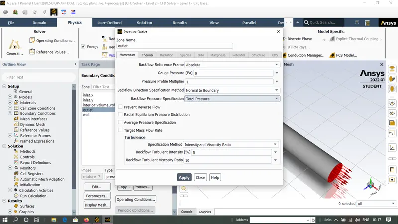
> Also check the boundary conditions for the outlet portion of the tee.
Setting up physics > cell Zones > boundaries > select outlet > type > pressure outlet > edit > pressure outlet > Gauge pressure as Zero >ok.
STEP 5 :
> Used to measure the some physical quantities such as avg temp and standard deviation after the solution has been solved.
Solution > Definitions > Area Weighted average > surface report variable > Field variable > Temperature > select face as outlet > create > select report file ,report port,frequency as 1 > ok.
> Frequency as 1 means the simulations will be occur for every itertion.
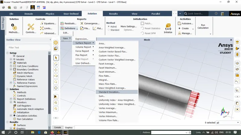
> For mixing problem to check the efficiency of mixing use surface based standard deviation.
Solution > Definitions > edit > Surface report definition > field variable as temperature > select face as outlet > create > select report file ,report port,frequency as 1 > ok.
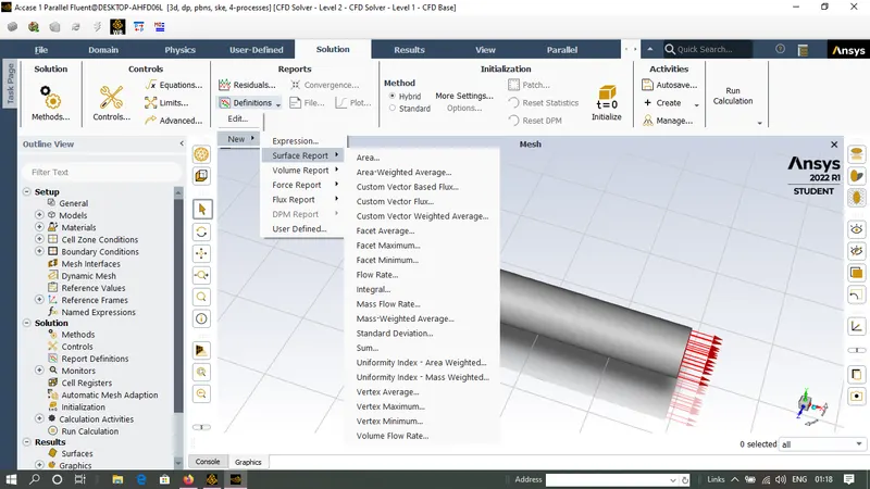
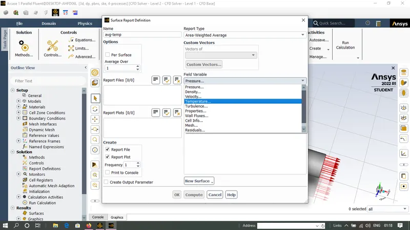
crete the report for the standard deviation of temperature at outlet.
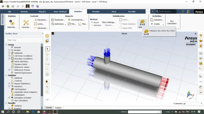
Hybrid initialization process used as a potential flow solver to compute the approximate value for velocity and pressure.
Solution > initialization > click on t = 0 initialize > Run calculation > number of iterations as 200 > click on calculate > diifrent plots will appear and the initilization will take some time.
:
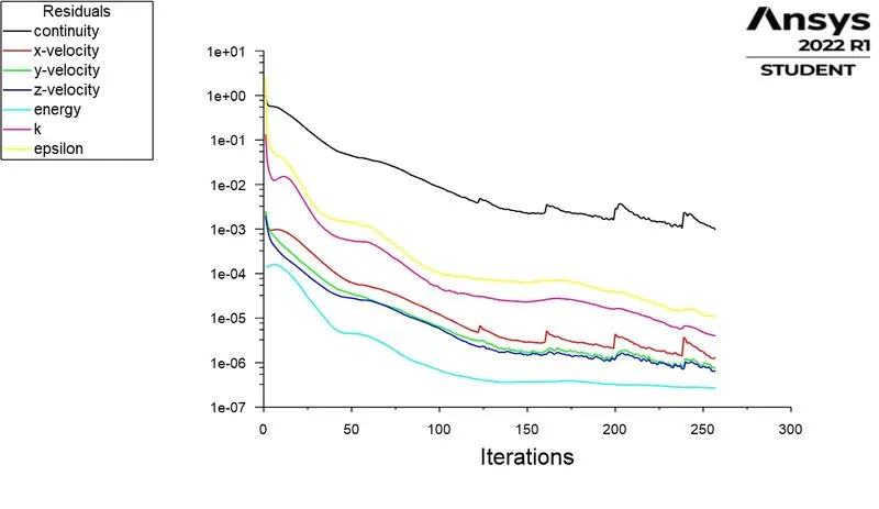
After performing the solution the Scaled Residuals for the short tee with momentum ratio of 2 are shown below.
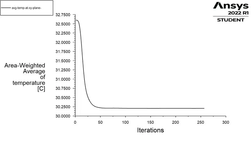
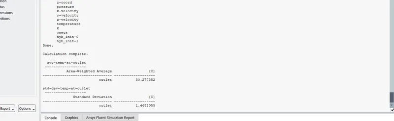
> Average temperature for short tee with momentum ratio of 2.
> Standard deviation for short tee having momentum ratio of 2.
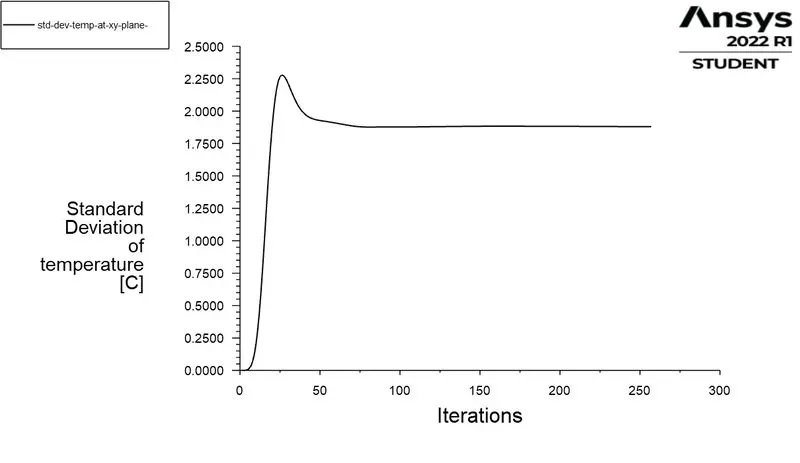
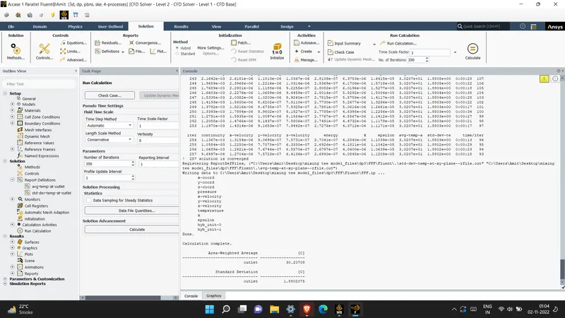
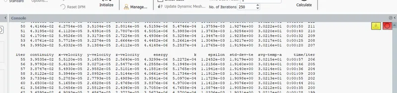
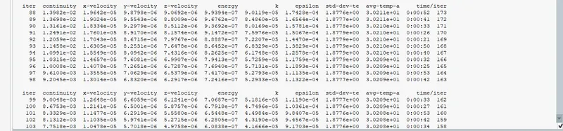
NOTE : From the above scaled residuals we can say that almost all the plots are converged after 180 to 220 iterations.From the above simulation in Case 1 we have observed that the residual plots took nearly 180-220 iterations to converge, area-weighted average of temperature plot took nearly 55 to 60 interations to converge and standard deviation of temperature took nearly 92 to 100 iterations to converge.
NOTE:
We use the FVM(finite volume method) to deicribe the partial diffrential equations and solve it and when we solve the function it might not be evaluate to zero,it might actually evaluate to something really small so these really small quantities are called as residuals.
STEP 8: Perform the post processing operations.
> Make sure to close the ansys fluent to avoid the license issue and then open the post processing tool.
Project schematic > fluid flow fluent > Results .
Cases > FFF > volume > untick all the box except wall volume > Rendor > apply some transparency > Apply.
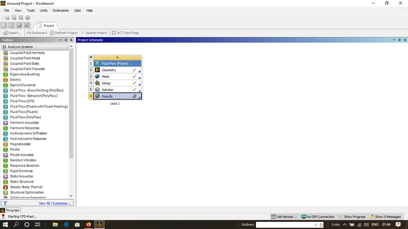
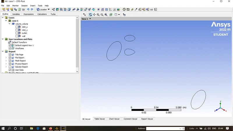
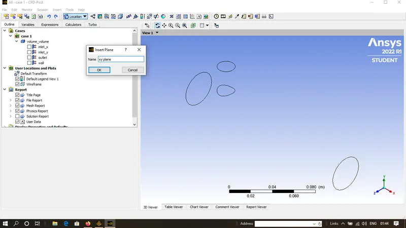
> Create the xy plane.
Insert > Location > plane > xy plane > z=0 > ok.
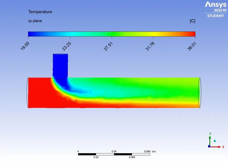
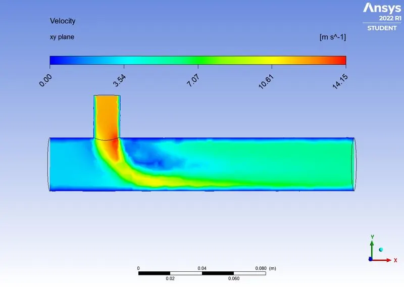
> Create the contors for the velocity and Temperature distribution.
To create the temperature contors use the layout as mentioned below.
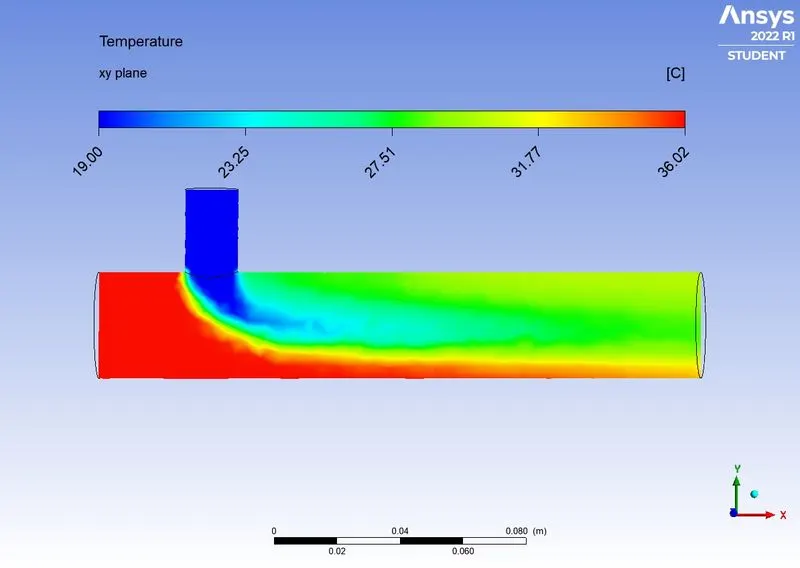
click on xy plane > details of xy plane > color > mode as variabe > select temp as variable > apply.
> To create the velocity contor use the layout.
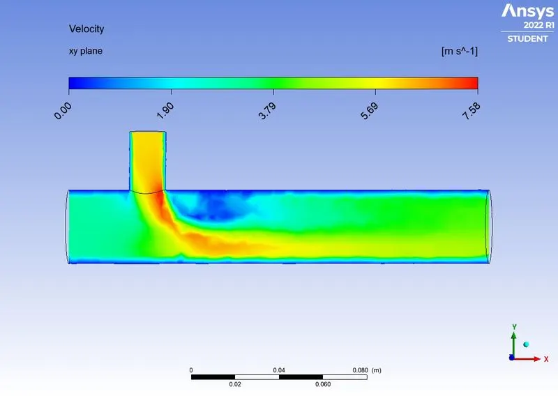
click on xy plane > details of xy plane > color > mode as variabe > select velocity as variable > apply
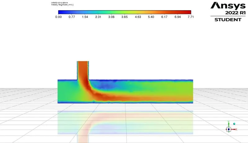
> to create the contor for the velocity vector use the layout.
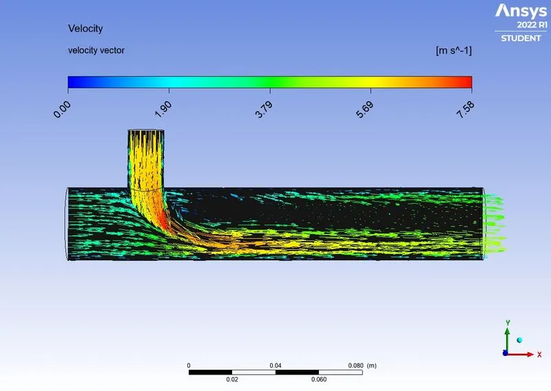
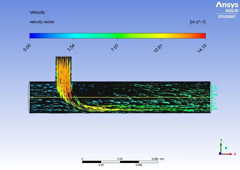
click on vector denoted by three arrows at upper side of the screen > assign name as velocity vector > details of velocity vector > under geometry tab select location as xy plane > select mode as variable > select variable as velocity > apply.
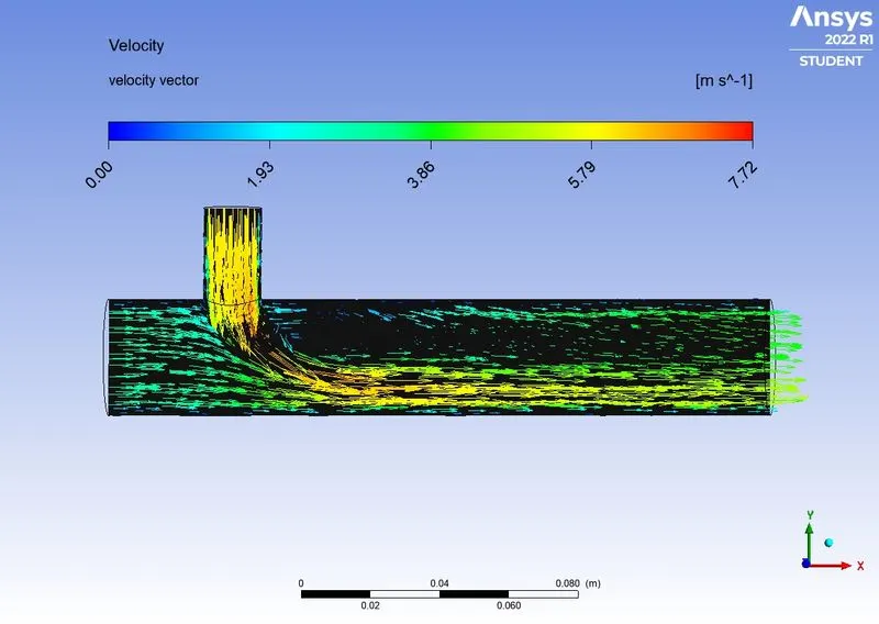
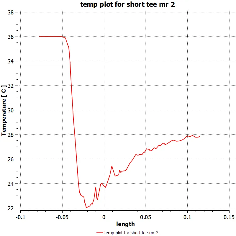
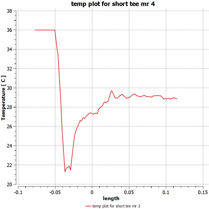
> Create the temp plot for short tee for momemtum ratio of 2.To create the plot first create the line using line coomand similary as we create the plane.
select chart option present at the rendor
assign name as temperature plot for case 1
Go to details of temperature chart for case1
In general tab give title name for the plot as temp plot for short tee with mr 2.
In data series tab give the name for the plot as temp plot fot short tee mr 2.
In x-axis tab give length as x-axis.
In y axis tab select temperature for the y-axis
press Apply.
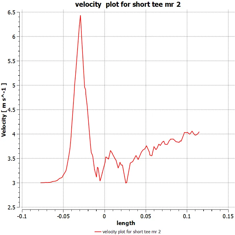
> Create the velocity plot for short tee for momemtum ratio of 2.To create the plot first create the line using line command similary as we create the plane.
select chart option present at the rendor
assign name as velocity plot for case 1
Go to details of velocity chart for case1
In general tab give title name for the plot as velocity plot for short tee with mr 2.
In data series tab give the name for the plot as velocity plot fot short tee mr 2.
In x-axis tab give length as x-axis.
In y axis tab select velocity for the y-axis
press Apply.
Case 2:
Parameters:
| Length | Short |
| Momentum Ratio | 2 |
| Hot air velocity with temperarure | 3m/s ; 36oC">36oC |
| Cold Air velocity with temperature | 6m/s ; 19oC">19oC |
| Element Size | 5mm |
| Number of Elements | 14255 |
| Turbulence Model | K-omega (SST) |
> right click on fluid flow > select duplicate > go to setup > select viscous model as k-omega sst model.
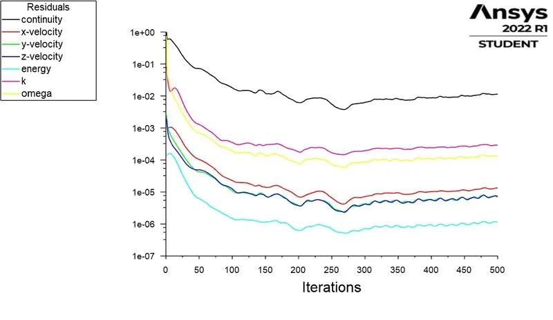
> Residual plot for short tee with mr 2 with turbulence model as k omega.
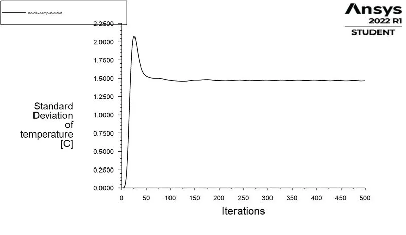
> Standard deviation for short tee with mr 2 having turbulence model as k-omega sst.
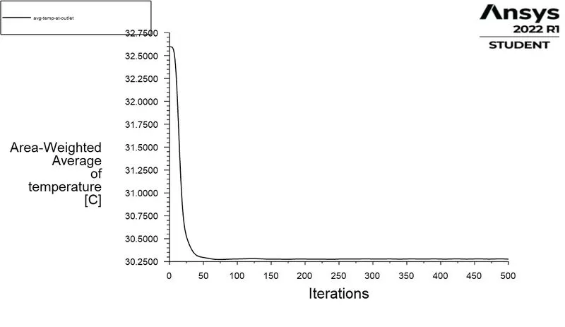
> Average temperature for short tee with mr 2 with turbulence model as k omega sst model.
POST PROCESSING:
> Tenperature plot:
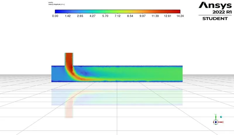
> Velocity plot:
> Velocity vector:
> Variation of temperature along the length.
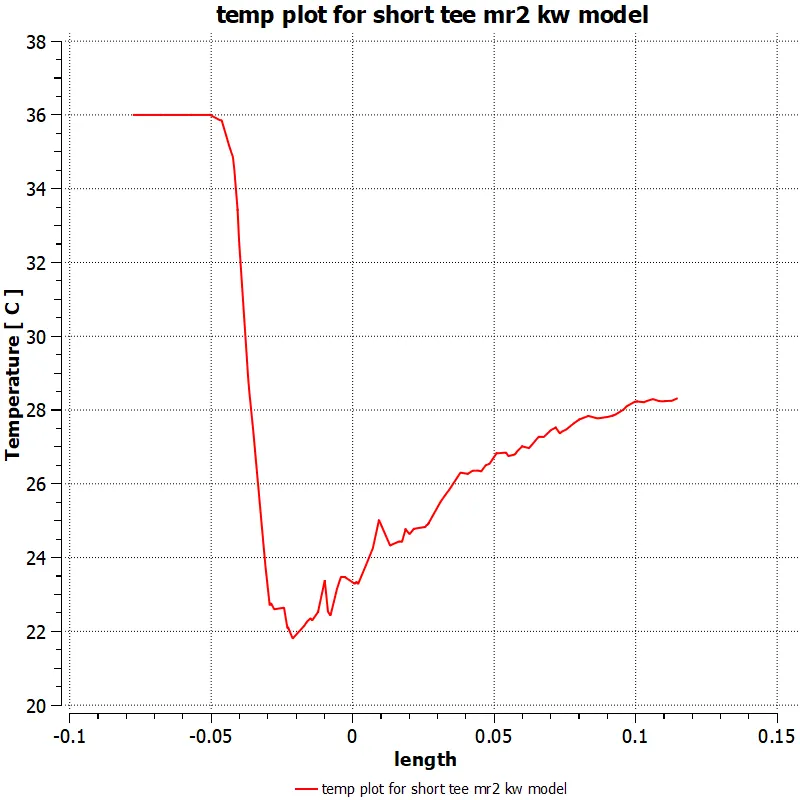
> Variation of velocity along the length of the mixing tee.
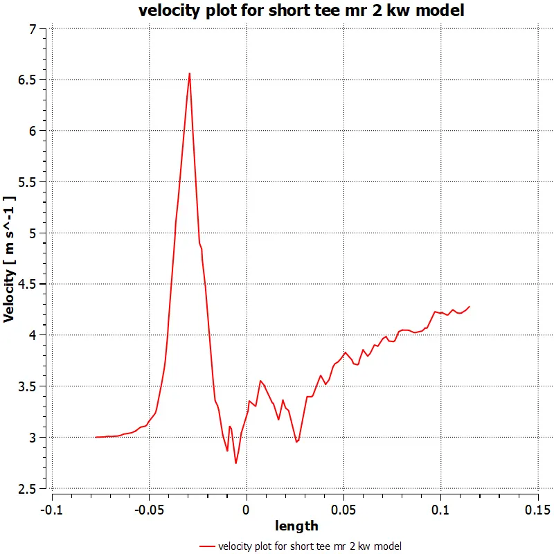
> From the above simulation in Case 2 we have observed that the residual plots took nearly 220 to 300 iterations to converge, area-weighted average of temperature plot took nearly 70-80 interations to converge and standard deviation of temperature took nearly 100-120 iterations to converge.
Comparison between case 1 and case 2:
| Cases | Turbulence model | Momentum Ratio | Tee-Length | No. of Elements | Outlet Temperature(Area-weighted) | Standard Deviation of the outlet temperature | No. of Iterations |
| Case 1 | K-epsilon | 2 | Short | 14255 | 30.20 C | 1.88 | 180-220 |
| Case 2 | K-omega | 2 | Short | 14255 | 30.27 C | 1.47 | 220-300 |
Comments:
We can observe from the above comparison that the results obtained by both the turbulence model are almost the same except K-omega took more number of iterations to converge than the K-epsilon turbulence model. In other words, the K-epsilon turbulence model is more efficient than K-omega model in terms of time taken to complete the simulation.
So we are going to choose K-epsilon model for simulation of the rest of the cases left.
From now the complete table of the cases we need to peform is represented as
| Cases | Momentum Ratios | Length | Turbulent Model |
| Case 1 | 2 | Short | K-epsilon |
| Case 2 | 2 | Short | K-omega |
| Case 3 | 4 | Short | K-epsilon |
| Case 4 | 2 | Long | K-epsilon |
| Case 5 | 4 | Long | K-epsilon |
Case 3:
Parameters:
| Length | Short |
| Momentum Ratio | 4 |
| Hot air velocity with temperarure | 3m/s ; 36oC |
| Cold Air velocity with temperature | 12m/s ; 19oC |
| Element Size | 5mm |
| Number of Elements | 14255 |
| Turbulence Model | K-epsilon (standard) |
> right click on the fluid fluent of the case 1 and select duplicate option and then select setup or Ansys fluent tool where change the boundary conditions for the inlet y. Give velocity as 12m/s and dont change other parameters.
Initialize the simulation and then run the simulation for 250 iterations.
Solving:
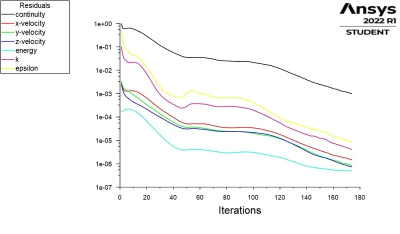
Scaled residulas for short tee having momentum ratio of 4.
 st
st
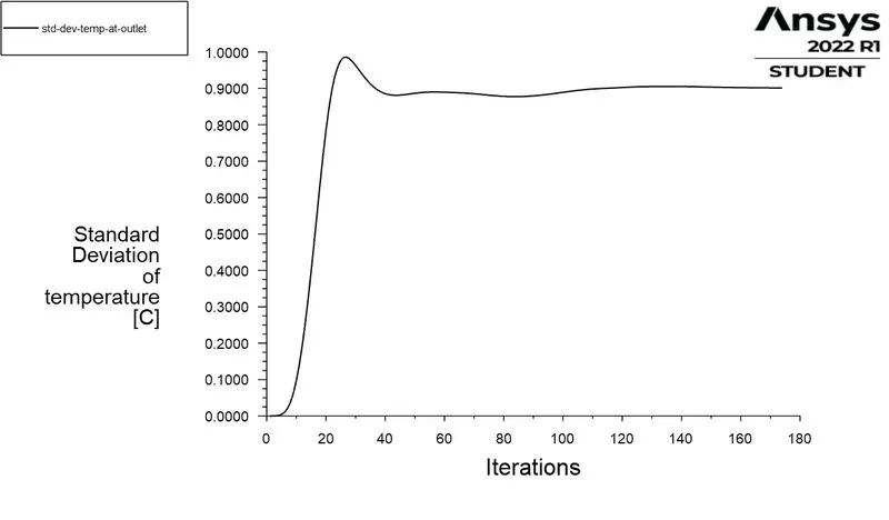
> Standard deviation of temperaure at outlet for short tee.
> Average temperature for short tee with momentum ratio of 4.
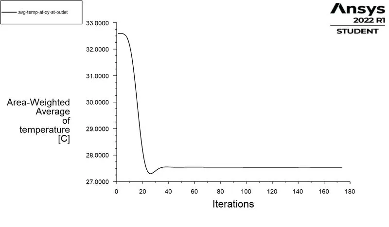
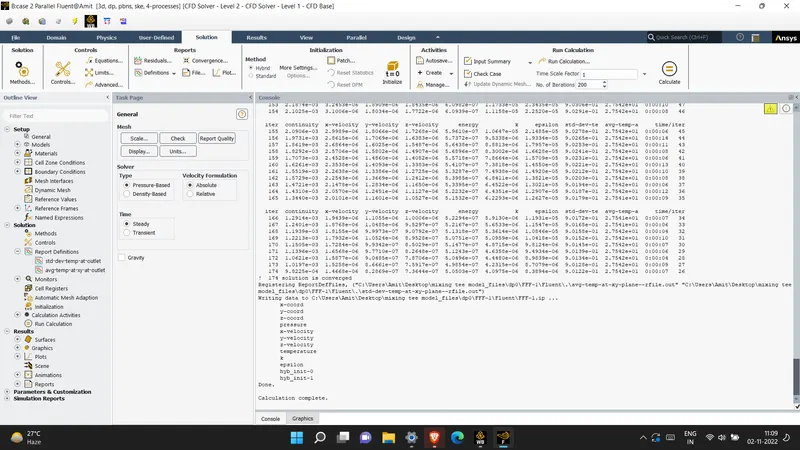
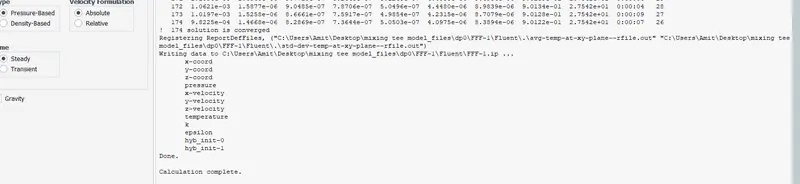

> The solution is converged after 174 iterations as shown in the above image.
> POST PRCESSING:
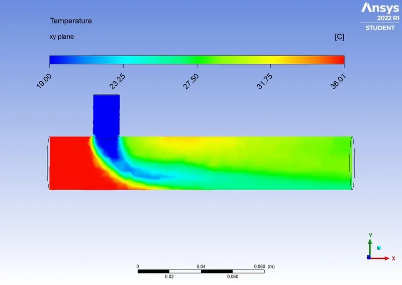
TEMPERATURE :
> VELOCITY :
> VELOCITY VECTOR:
> VARIATION OF TEMPERATURE ALONG THE LENGTH OF THE PIPE:
> VARIATION OF VELOCITY ALONG THE LENGTH OF THE PIPE:
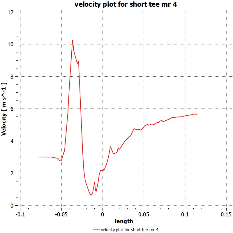
Here the velocity is suddenly inccresed due to the cold fluid has velocity which is four times greater than the velocity for the hot fluid.
Case 4:
Parameters:
| Length | Long |
| Momentum Ratio | 2 |
| Hot air velocity with temperarure | 3m/s ; 36oC |
| Cold Air velocity with temperature | 6m/s ; 19oC |
| Element Size | 5mm |
| Number of Elements | 14255 |
| Turbulence Model | K-epsilon (standard) |
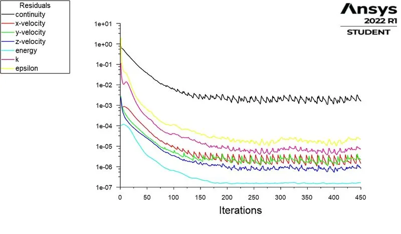
> RESIDULS PLOT AT OULET:
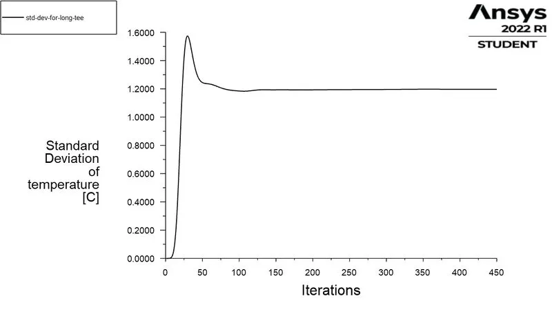
> STANDARD DEVIATION:
> AVERAGE TEMPERATURE:
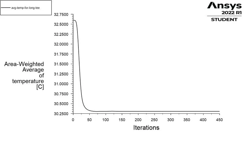
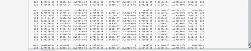
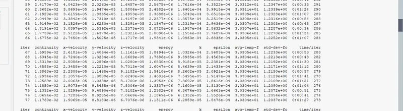
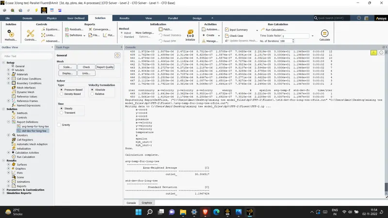
Solution is converged between 150 to 175 iterations while the average temperature is converged between 67 to 70 iterations while the standard deviation of temperature is converged between 120 to 130 iterations.

> POST PROCESSING:
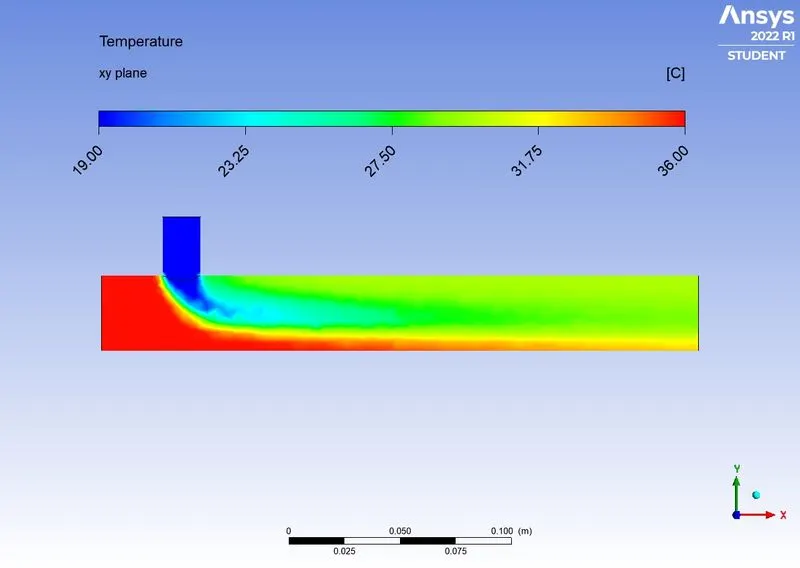
TEMPERATURE PLOT:
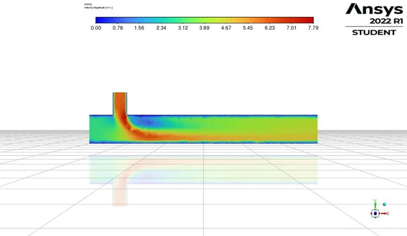
> VELOCITY PLOT:
Case 5:
Parameters:
| Length | Long |
| Momentum Ratio | 4 |
| Hot air velocity with temperarure | 3m/s ;36oC |
| Cold Air velocity with temperature | 12m/s ;19oC |
| Element Size | 5mm |
| Number of Elements | 14255 |
| Turbulence Model | K-epsilon (standard) |
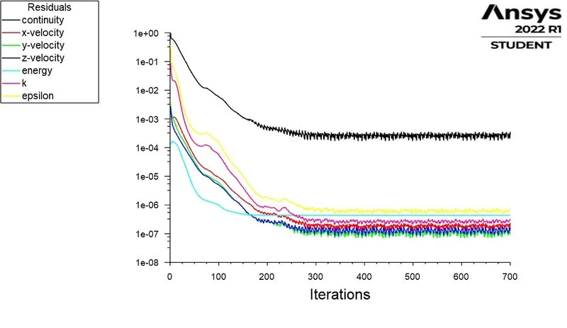
> Residuals plot:
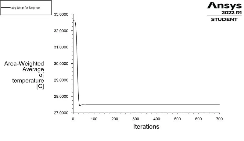
> Average temperature for long tee with momentum ratio of 4.
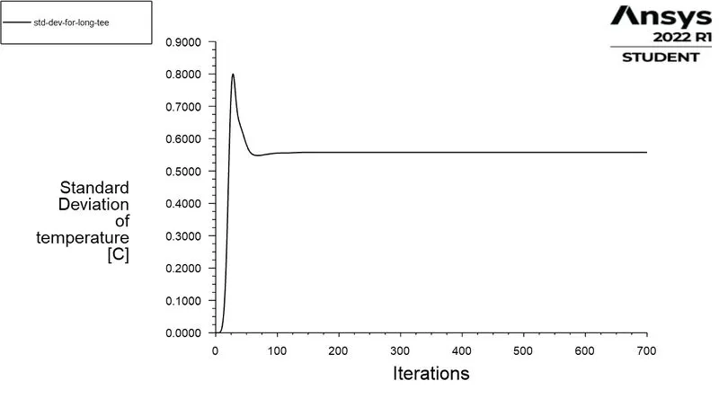
> Standard deviation :

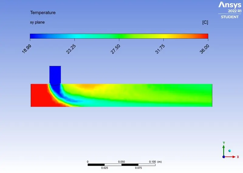
POST PROCESSING:
TEMPERATURE PLOT:
> VELOCITY PLOT:
Analytical Solution of the mixture:
The temperature at the outlet of the tee-pipe is given as,
Given data,
Thot=36oC,andTcold=19oCThot=36oC,andTcold=19oC
Momentum ratio is 4,
Vhot=3m/s,Vcold=12m/sVhot=3m/s,Vcold=12m/s
mhot=ρAhotVhot=1.225×225.9131×3=3313.0959kg/smhot=ρAhotVhot=1.225×225.9131×3=3313.0959kg/s
mcold=ρAcoldVcold=1.225×225.9131×6=3320.9225kg/smcold=ρAcoldVcold=1.225×225.9131×6=3320.9225kg/s
Tmixture=3313.0959×36+3320.9225×193313.0959+3320.9225Tmixture=3313.0959×36+3320.9225×193313.0959+3320.9225
Tmixture=27.48oC
Observations:
| Cases | Turbulence model | Momentum Ratio | Tee-Length | No. of Elements | Outlet Temperature(Area-weighted) | Standard Deviation of the outlet temperature | No. of Iterations |
| Case 1 | K-epsilon | 2 | Short | 14255 | 30.20 C | 1.88 C | 180-220 |
| Case 2 | K-omega | 2 | Short | 14255 | 30.27 C | 1.47 C | 220-300 |
| Case 3 | K-epsilon | 4 | Short | 14255 | 27.54 C | 0.90 C | 174 |
| Case 4 | K-epsilon | 2 | Long | 14255 | 30.30 C | 1.19 C | 350 |
| Case 5 | K-epsilon | 4 | Long | 14255 | 27.48 C | 0.55 C | 700 (Solution not converged) |
- K-epsilon turbulence model is more time efficient than the K-omega turbulence model.
- In case 3 where the momentum ratio is 4 the solution is converged at 174 no. of iterations whereas in case 5 where the tee-length is long, the solution obtained is exactly equal to the analytical solution and has the lowest standard deviation of temperature. But the solution does not achieve steady state even at 700 no. of iterations.
- In case 4, the tee-length is long and the solution gets closest to the analytical solution with momentum ratio 2.
- After observing all these facts from the simulation we came to a conclusion that although the no. of iterations taken by the longer tee-length is more than the shorter tee-length but the more accurate results are obtained in case of the longer tee-length instead of shorter tee-length.