Week 1- Mixing Tee
Aim:
To set up steady-state simulations for two versions of the mixing tee.
One of them is longer than the other and compares the mixing effectiveness when the hot inlet temperature is 360C & the Cold inlet is at 190C.
Mixing Tee:
Mixing tee is a device used in different industries to mix the chemicals, fluids, etc in an air conditioner it is used to mix the outside air and conditioned air. steady-state conditioned simulations were also performed using the mixed-tee model.
Mixing Tees are utilized efficiently to mix two or more fluid streams into one combined stream. In this process both Mass and Heat transfer takes place. These are mainly used in HVAC applications, Refrigeration, etc.
In this assignment, we are going to analyze a mixing tee. Hot air is flowing through a mainstream pipe. Cold air enters through the tee, where these two hot and cold fluids mix along the pipe.
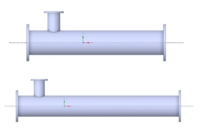
Cases:
Case 1: Short mixing tee
Case A: hot inlet velocity of 3 m/s, Momentum ratio of 2.
Case B: hot inlet velocity of 3 m/s, Momentum ratio of 4.
Case 2: Long mixing tee
Case C: hot inlet velocity of 3 m/s, Momentum ratio of 2.
Case D: hot inlet velocity of 3 m/s, Momentum ratio of 4.
Momentum ratio = velocity at cold inlet / velocity at hot inlet
Basic Procedure for all the cases:
Here we are simulating a long mixing tee Case 2(C): hot inlet velocity of 3 m/s, Momentum ratio of 2
Open ANSYS Workbench and import Fluid Flow (Fluent) to the workspace. Fluid flow system (fluent) from the system given in the toolbox on the left side. to add this system we drag and drop it into the project schematic window. Then we can see it in various steps we start with the geometry.
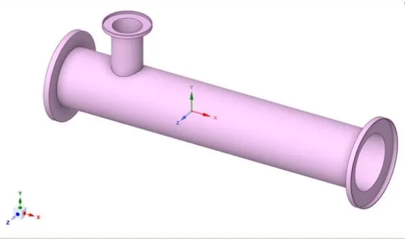
Double click on Geometry it will automatically redirect to space claim where we can import our Tee cad model. We open the geometry that we have for the Mixing Tee. we can see it in the GUI as shown below after importing the CAD model extract the Volume of the fluid domain using the volume extract command. This extracted fluid domain is going to represent a fluid space in physical calculations. Hide the outer shell (CAD model) and suppress it for physics. This whole process is simply called CAD clean-up.
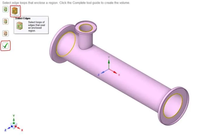
Extract the flow volume where the fluid flow occurs for this we will go to the Prepare tab and select the volume extract button. Now to extract the fluid we will cap the three openings in the shell using the edge selection tool and then click on the three edges as shown in the following figure after that click on the right tick mark to extract the volume.
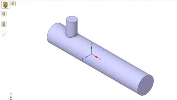
Now we can see that the fluid volume has been extracted and is visible in the tree on the left side. also, we will be unchecking the box for the Shell1 and suppress it for physics by right-clicking on it and selecting the suppress for physics option. Then we get our desired volume.
Now we will be closing the SpaceClaim and it will be updated in the workbench. we move on to the next step which is meshing by double-clicking on the Mesh.
Mesh:
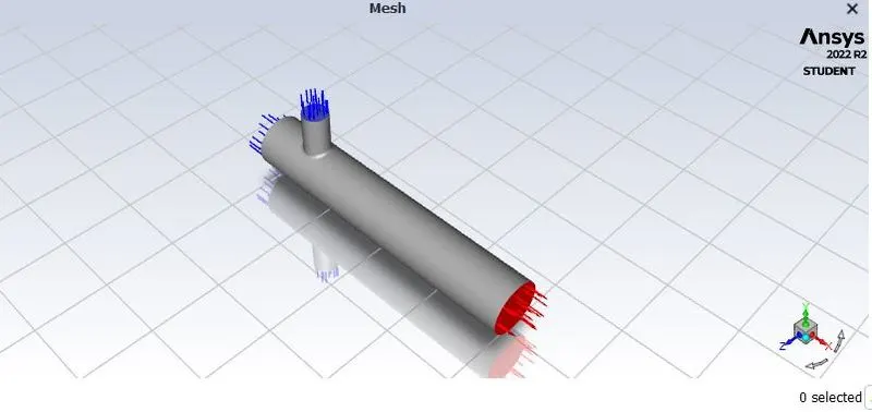
Update the Geometry before opening the mesh. Open mesh first verifies that no external CAD model is not there except the Fluid domain. Then will be naming the parts of the model by using named selection which can be done by selecting the part to be named and then right click on the part and selecting the named selection option or using N as the shortcut. The named sections are shown in the following images.
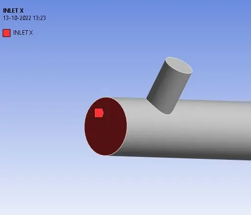
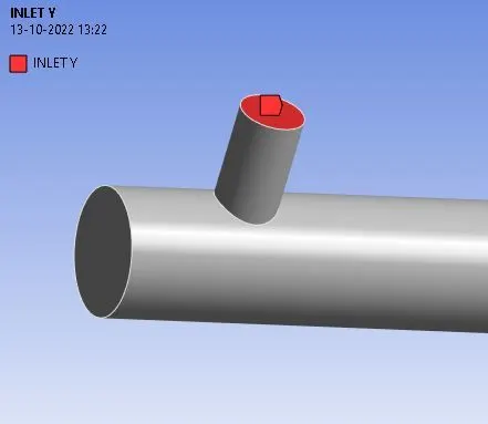
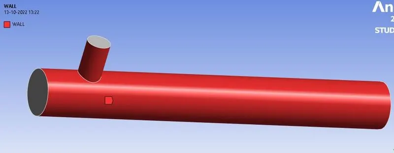
Now moving to the meshing part we will be first meshing our model by keeping the default values for all the parameters in Ansys meshing. So here we select Mesh from the tree using the right mouse button and select the generate mesh option and it will be generating the mesh.
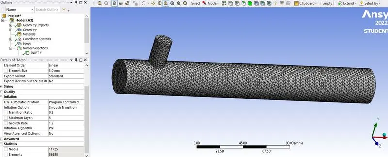
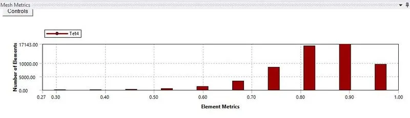
Here it is seen that the minimum mesh quality is 0.27 which is more than the value of 0.05 so our mesh is pretty good and we can use this mesh for our simulation process.
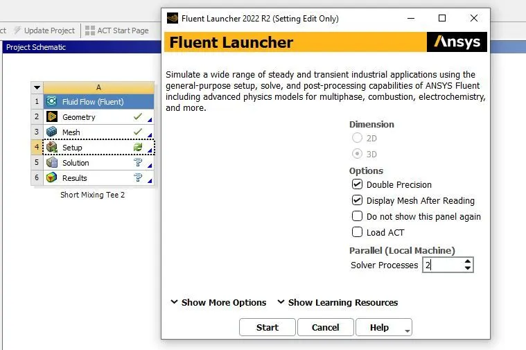
Now moving to the next step from the workbench which is the setup that we are in the fluent, so double clicking setup will open a fluent launcher, there we first check the double precision box and give 2 processors for parallel solvers processes.
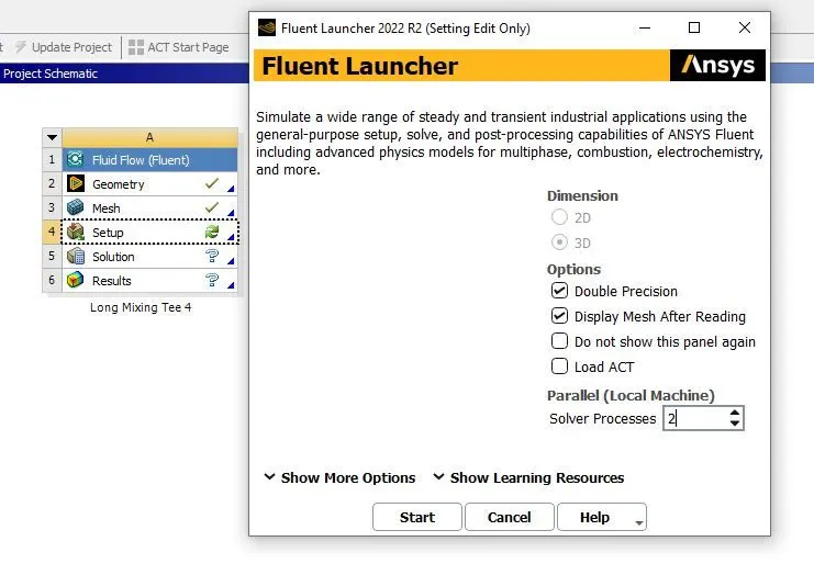
After starting the fluent our mesh model will load up inside the fluent GUI.
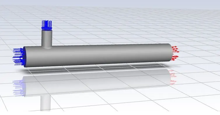
first, we will be performing the mesh check from the domain tab in the ribbon, it will give the output in the console as shown.
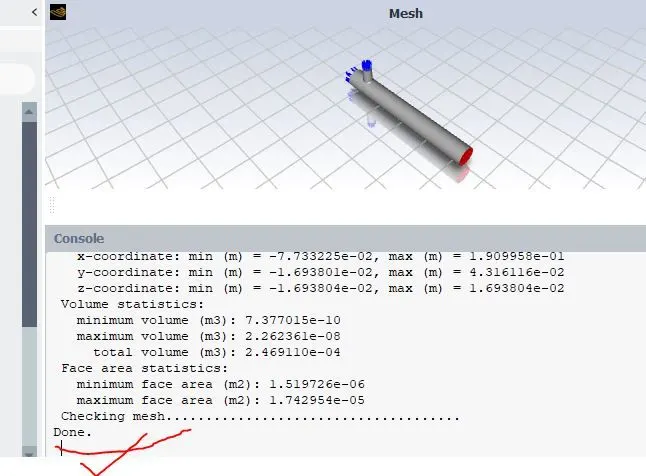
This means our mesh is good. we will be using a pressure-based steady solver.
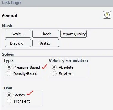
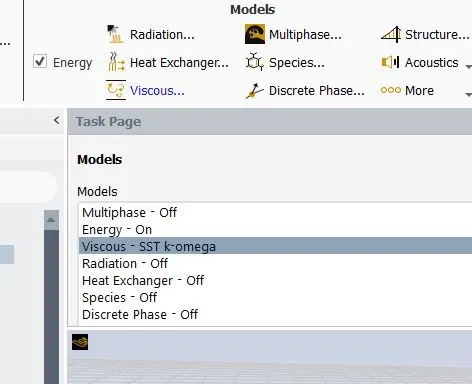
Moving to the physics tab to set up the physics of the simulation. We will check the energy box under the model's menu. and then change the viscous model to the standard k-OMEGA model with SST wall conditions.
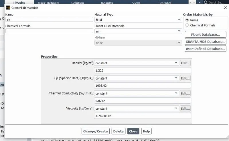
We set the material as Air.
Set the boundaries from the boundaries option under the zones menu.
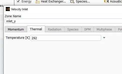
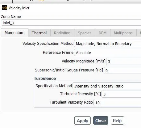
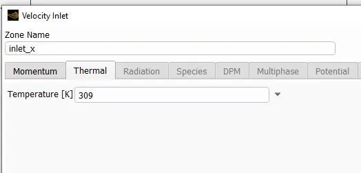
Using the momentum ratio as 2 and as our hot inlet velocity is 3 m/s then the cold inlet velocity will become 6 m/s, also the temperature of the cold inlet will be 19 degrees Celcius and for the hot inlet, the temperature will be 36 degrees Celcius as given in the problem definition.
For cold inlet velocity:
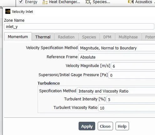
For hot inlet velocity:
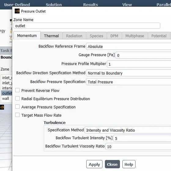
For pressure outlet:
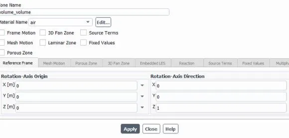
Also, we will make sure that our cell zone conditions are set to air as the material.
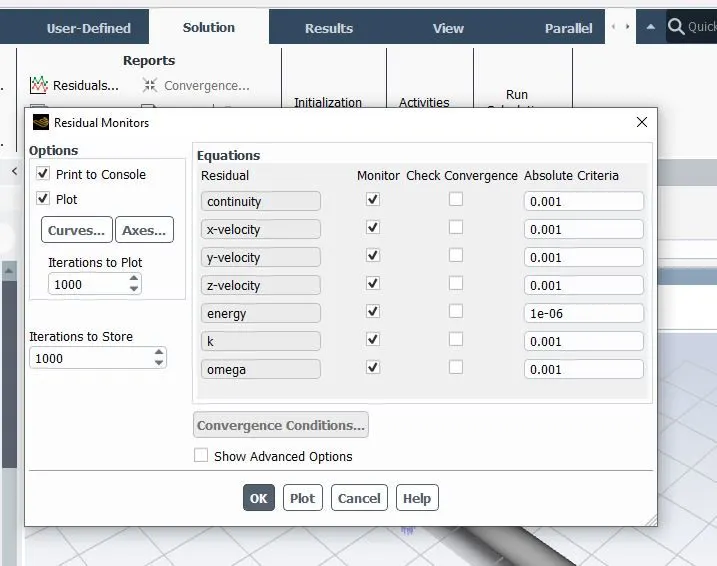
Now moving to the solution tab to set up the solver, we will first uncheck for convergence for all the residual parameters by going to the residual monitors under the reports menu.
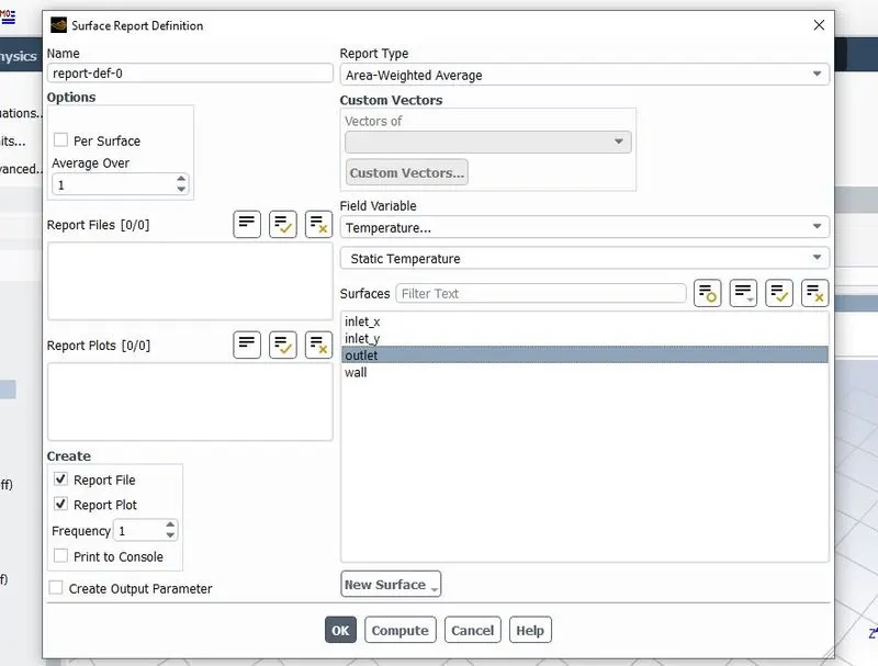
After this, we set up a new report definition to measure the surface report of the area-weighted average of the temperature at the outlet.
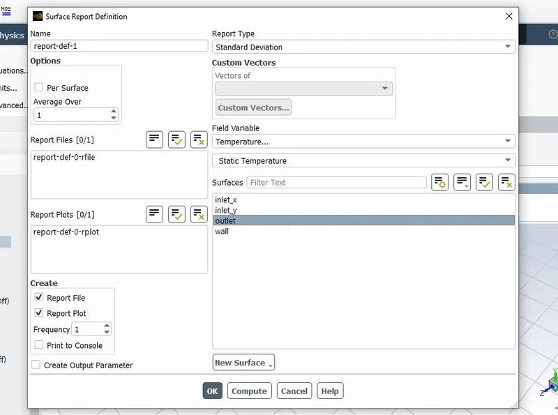
Now we will set up one more report definition for the surface report of the standard deviation of the temperature at the outlet.
Now we will be initializing our simulation by selecting the initialize button from the initialization menu and we have set the method as a hybrid which was the default method.
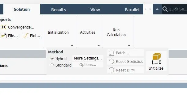
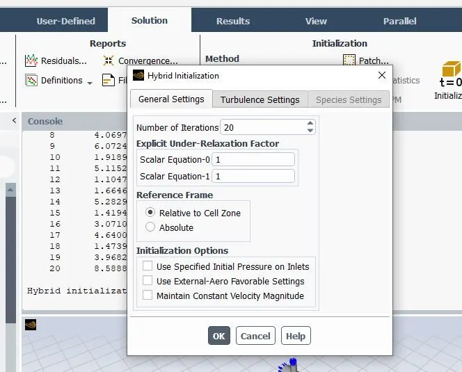
After the initialization, we were getting a warning in the console. so we go to the MORE settings in the initialization menu and change the number of iterations to 20 from the default value of 10.
Now we will set the number of iterations to 300 and hit calculate under the run calculation menu to simulate our solution.
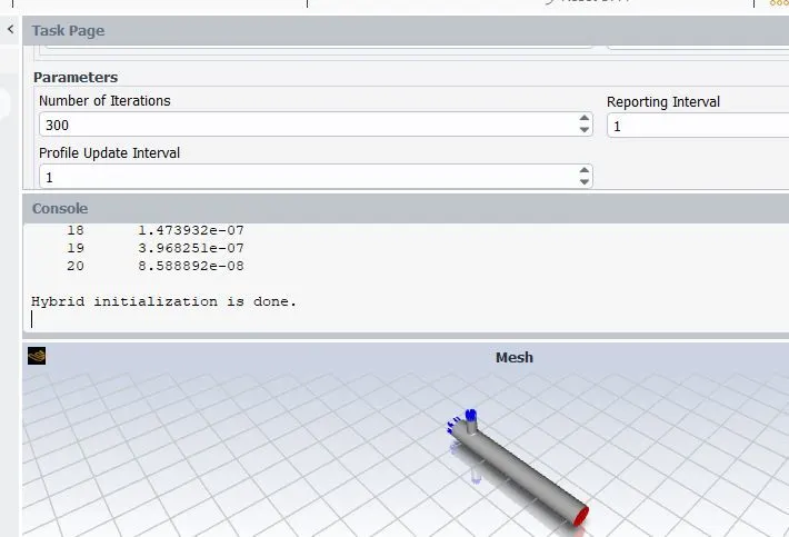
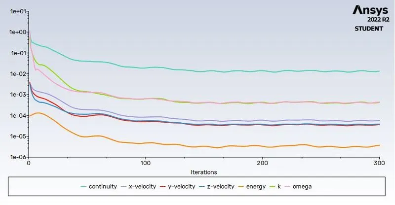
After 300 iterations our calculation is completed, and we can see that the residuals are following a similar pattern after about 200 iterations.
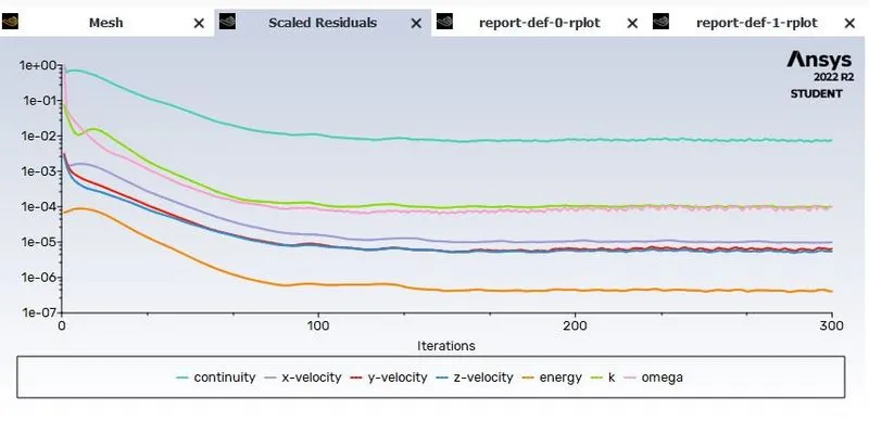
Here we can see that the energy residuals are almost a straight line after 200 iterations so we can say that our solutions have converged at about 200 iterations.
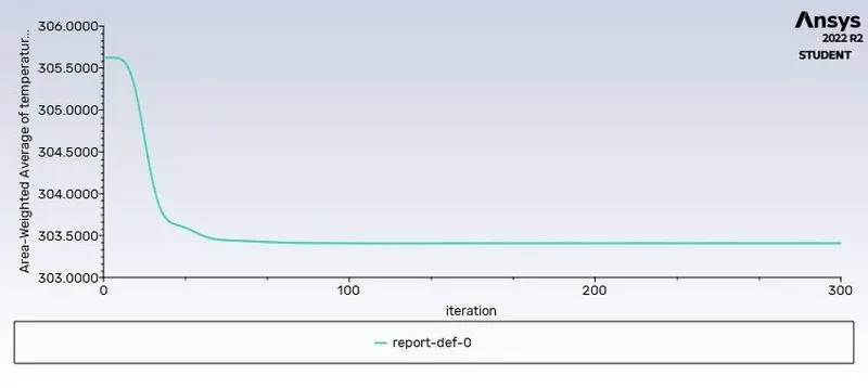
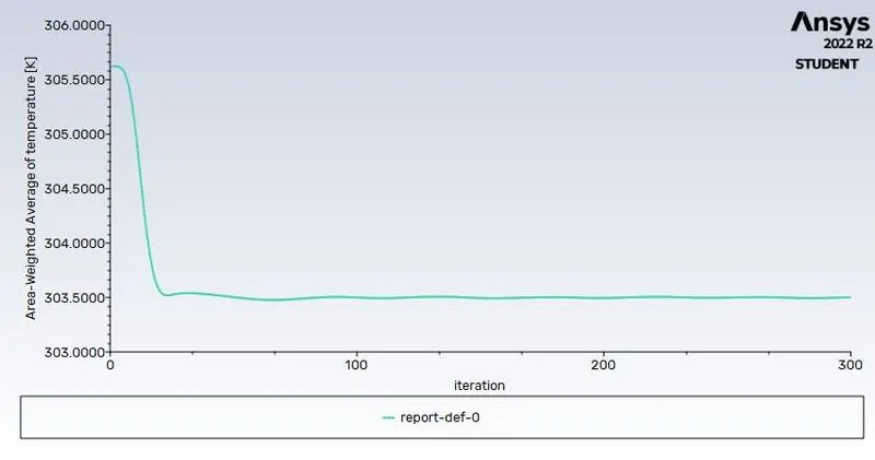
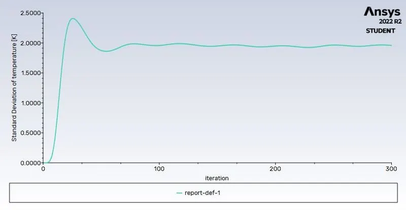
From the area weight average temp plot at the outlet, we can see that we get a converged value at 100 iterations. And form the standard deviation of temperature at the outlet we can say that the values of standard deviation have converged at about 150 iterations.
The area-weighted average temperature at the outlet is 30 degrees Celcius.
So now we will be post-processing our solution in CFD post.
In the CFD post, we will be creating a temperature contour at the midplane of the mixing Tee so we can see the temperature along and across the pipe.
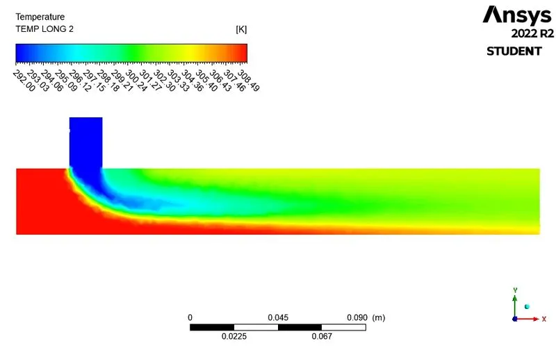
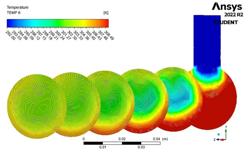
In the CFD post, we will be creating a Velocity contour at the midplane of the mixing Tee so we can see the temperature along and across the pipe.
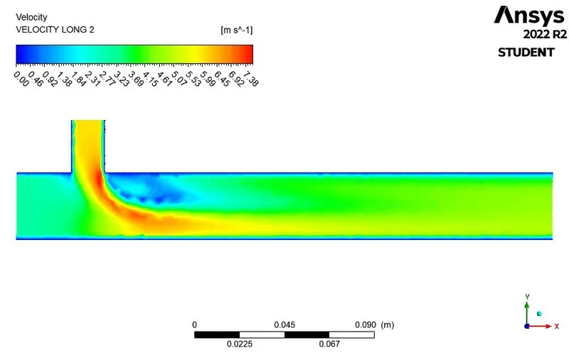
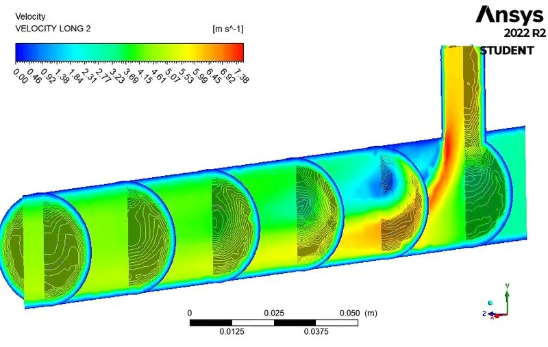
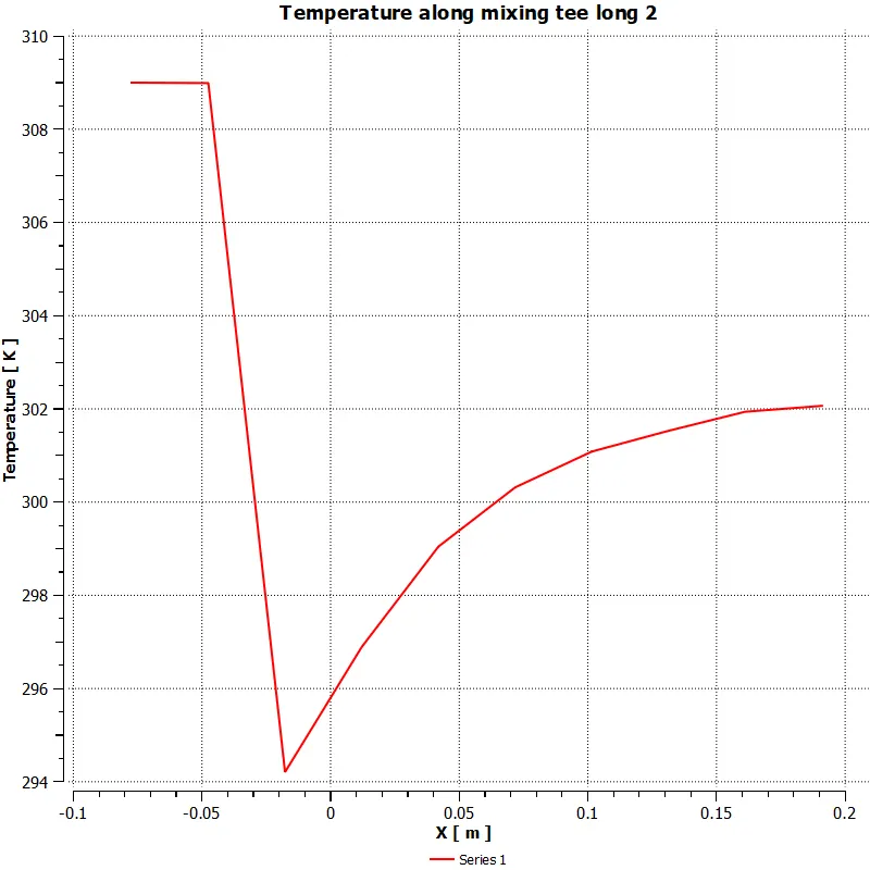
Various plots related to the solution are shown below:
Temperature plot along the pipe.
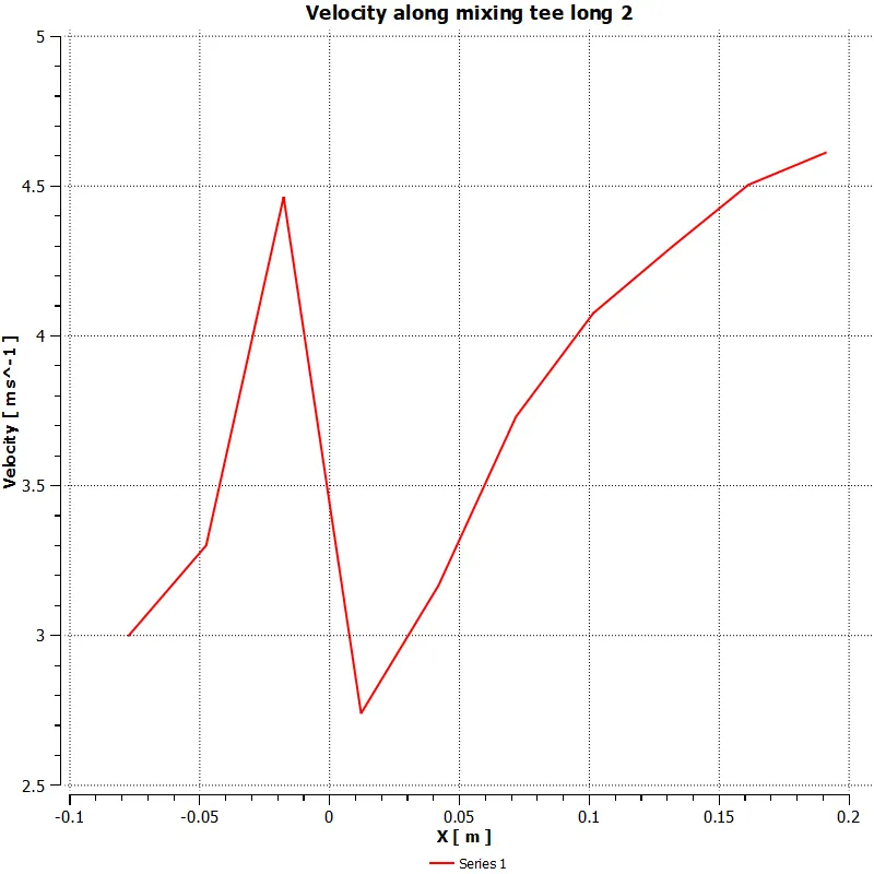
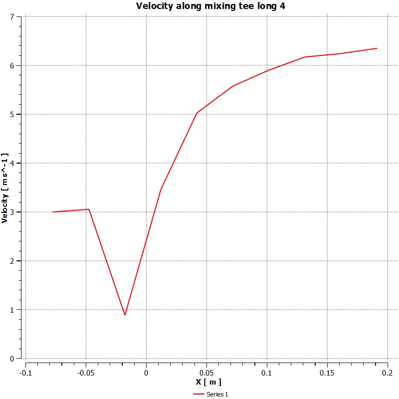
Velocity plot along the pipe.
Here we are simulating a long mixing tee Case 2(D): hot inlet velocity of 3 m/s, Momentum ratio of 4
Using the momentum ratio of 4 and as our hot inlet velocity is 3 m/s then the cold inlet velocity will become 12 m/s, also the temperature of the cold inlet will be 292 Kelvin and for the hot inlet, the temperature will be 309 Kelvin as given in the problem definition.
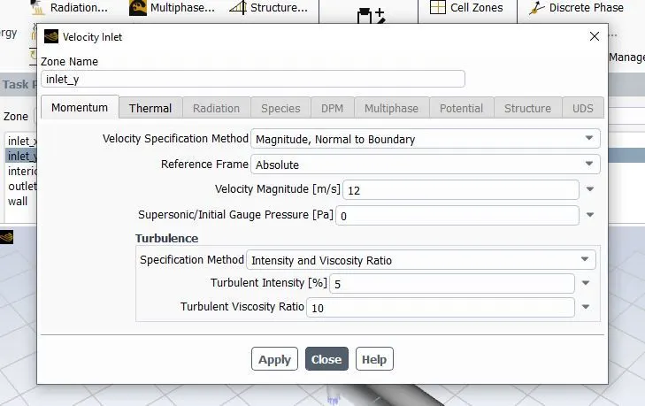
Everything is the same except the velocity of the cold inlet is 12 m/s.
Now we will set the number of iterations to 300 and hit calculate under the run calculation menu to simulate our solution.
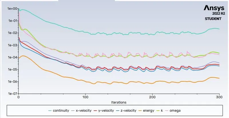
After 300 iterations our calculation is completed, and we can see that the residuals are following a similar pattern after about 220 iterations.
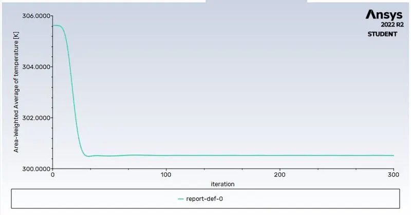
From the area weight average temp plot at the outlet, we can see that we get a converged value at 100 iterations.
And form the standard deviation of temperature at the outlet we can say that the values of standard deviation have converged at about 110 iterations.
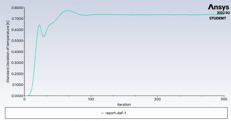
The standard deviation of temperature at the outlet is less that the shorter pipe.
So now we will be post-processing our solution in CFD post.
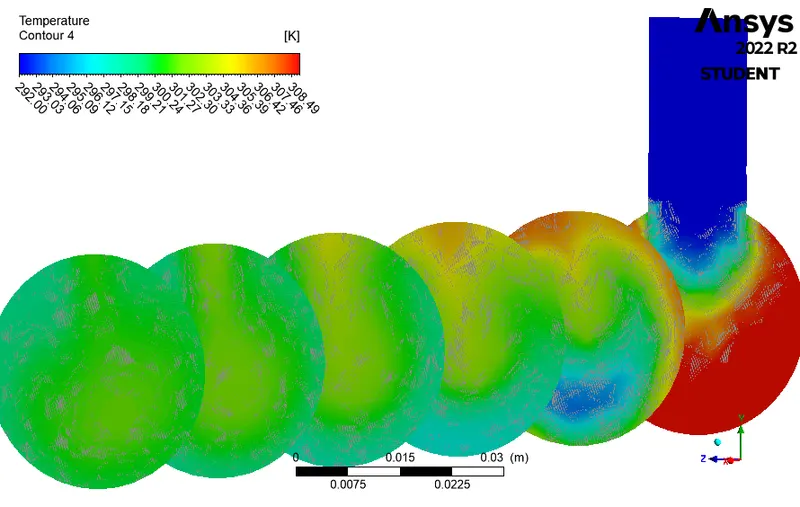
In the CFD post, we will be creating a temperature contour at the midplane of the mixing Tee so we can see the temperature along and across the pipe.
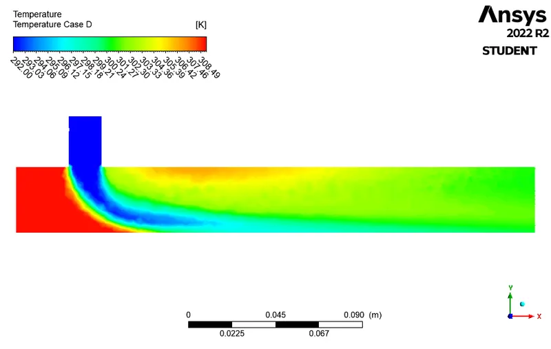
The temperature contour of is shows a well-mixed profile at the outlet and also the standard deviation is lowest in this case.
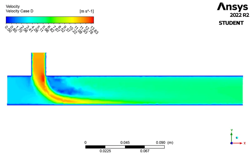
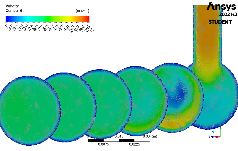
In the CFD post, we will be creating a Velocity contour at the midplane of the mixing Tee so we can see the temperature along and across the pipe.
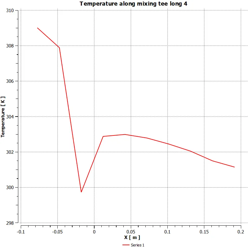
Various plots related to the solution are shown below:
Temperature plot along the pipe.
Velocity plot along the pipe.
SHORT MIXING TEE
Here we are simulating a long mixing tee Case 1(A): hot inlet velocity of 3 m/s, Momentum ratio of 2
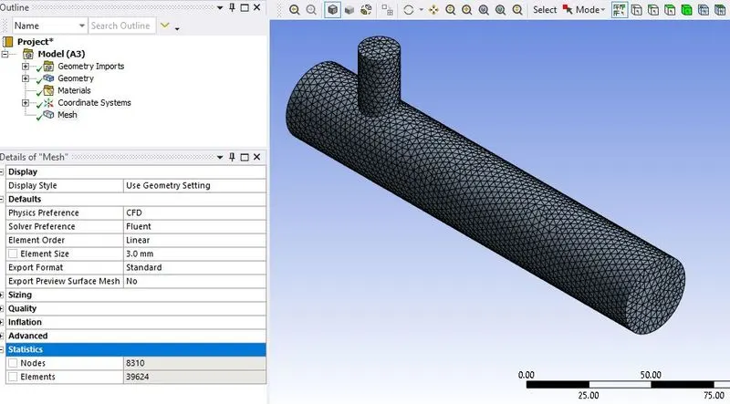
Now we will be simulation our case with the momentum ratio of 2 and so the new values of the cold and hot inlets will become 6 m/s and 3m/s respectively. We will be using the element size of 3 mm and the k-omega SST Model. The temperature of the inlets will be the same as earlier.
we will be generating the mesh with the element size of 3 mm and then loading it to Ansys fluent. While setting up the simulation the cold inlet velocity will be changed because the momentum ratio for this case is 2.
as the hot inlet velocity is fixed to 3 m/s then the cold inlet velocity will become 6 m/s. And the temperature at the cold inlet is 292 Kelvin and the temperature at the hot inlet is 309 Kelvin.
we are extracting the outer shell of geometry to smooth CFD mesh to continue, for we are following the procedure mentioned below
- open the Ansys workbench
- select Ansys fluent application in the workbench
- once the Ansys fluent is loaded it follows the workflow like geometry, mesh, setup, solution, results
- so select the geometry--->rightclick--->spaceclaim---->select
- once the SpaceClaim is loaded click on file------>open------>select step file------>ok
- go to prepare tab------>select volume extract------>select edge------>select correct edges------>confirm------>volume will be extracted------>on tree map select shell 1------>supress for physics
Pre-processing and solver setting
b) Mesh
- open mesh in the workbench
- give names like inlet, outlet, and walls for geometry by selecting a face, name selection
- geometry will be loaded automatically to generate some default mesh
- change the element size to 3 mm and update the mesh
- check the mesh element quality
Setup:
- After selecting set up we have to check double precision and no of cores.
- check the mesh report in the console.
- go to the physics tab, turn on the energy, go to viscous select k-omega(2-eqn) SST-ok.
- Click on materials--->select air as the fluid
- select boundary conditions--->inlet_x--->enter velocity--->3 m/s
- inlet_y--->velocity--->6 m/s
- go to solution tab select definitions --->new--->surface report--->area weighted average,standard deviation
- initialize with hybrid
- enter no of iterations like 300
- run the simulation--->calculate
- after simulation, we can see the plots like temperature, pressure vs length respect
Now we will set the number of iterations to 300 and hit calculate under the run calculation menu to simulate our solution.
After 300 iterations our calculation is completed, and we can see that the residuals are following a similar pattern after about 200 iterations.
From the area weight average temp plot at the outlet, we can see that we get a converged value at 90 iterations.
And form the standard deviation of temperature at the outlet we can say that the values of standard deviation have converged at about 150 iterations.
So now we will be post-processing our solution in CFD post.
In the CFD post, we will be creating a temperature contour at the midplane of the mixing Tee so we can see the temperature along and across the pipe.
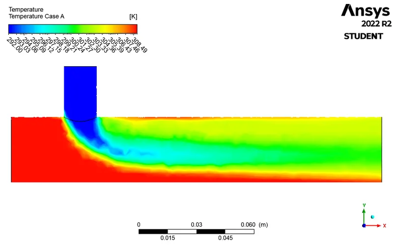
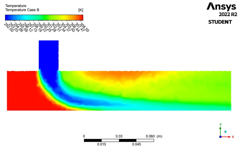
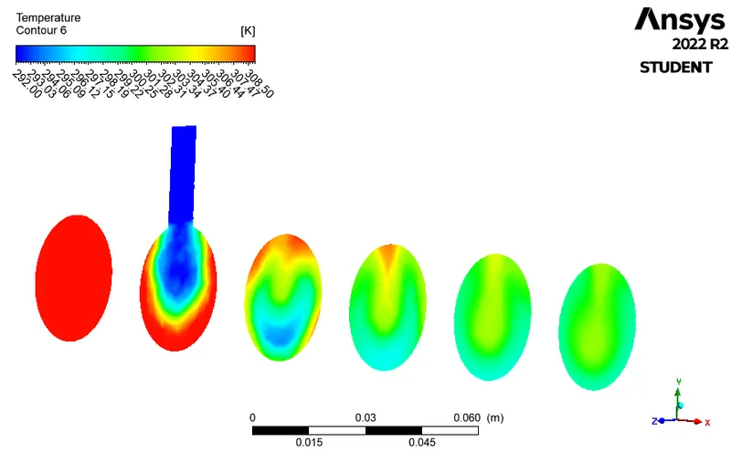
The temperature contour looks like it the not mixed more properly than compared to the longer pipe.
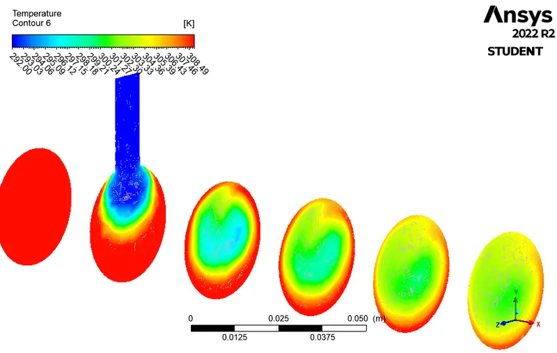
In the CFD post, we will be creating a Velocity contour at the midplane of the mixing Tee so we can see the temperature along and across the pipe.
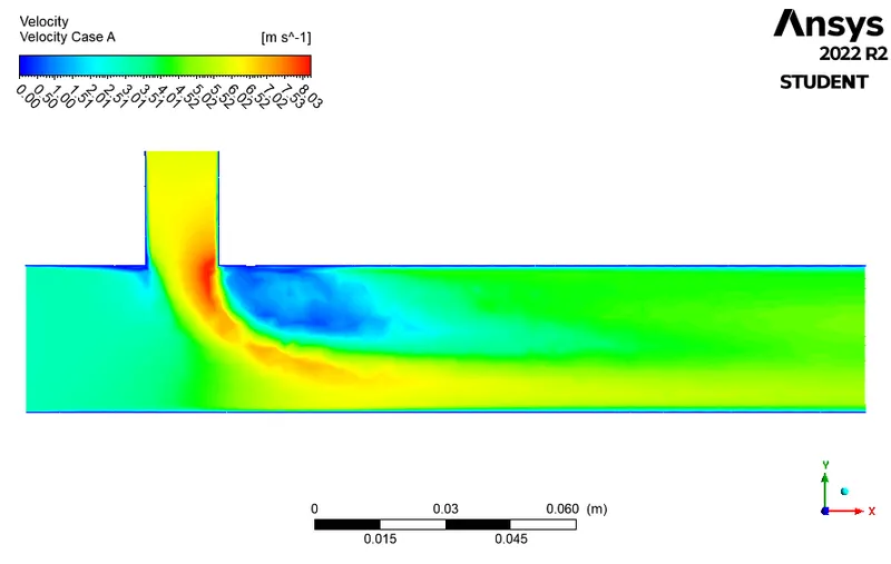
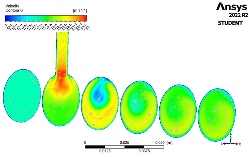
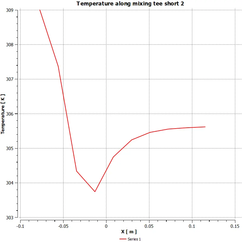
Various plots related to the solution are shown below:
Temperature plot along the pipe.
Velocity plot along the pipe.
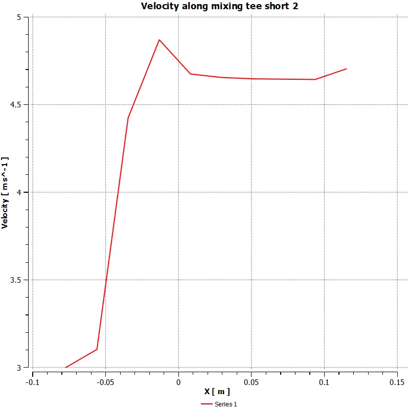
Here we are simulating a long mixing tee Case 1(B): hot inlet velocity of 3 m/s, Momentum ratio of 4
Now we will be simulation our case with the momentum ratio of 4 and so the new values of the cold and hot inlets will become 12 m/s and 3m/s respectively. We will be using the element size of 3 mm and the k-omega SST Model. The temperature of the inlets will be the same as earlier.
Now we will be changing the geometry of the mixing tee from a long length of pipe to a short length pipe. and the extracted volume. now we will be loading this geometry into the meshing to mesh and then we will mesh it with an element size of 3 mm. we will be generating the mesh with the element size of 3 mm and then loading it to Ansys fluent. While setting up the simulation the cold inlet velocity will be changed because the momentum ratio for this case is 4.
as the hot inlet velocity is fixed to 3 m/s then the cold inlet velocity will become 12 m/s. And the temperature at the cold inlet is 292 Kelvin and the temperature at the hot inlet is 309 Kelvin.
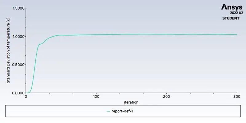
Now we will set the number of iterations to 300 and hit calculate under the run calculation menu to simulate our solution.
After 300 iterations our calculation is completed, and we can see that the residuals are following a similar pattern after about 200 iterations.
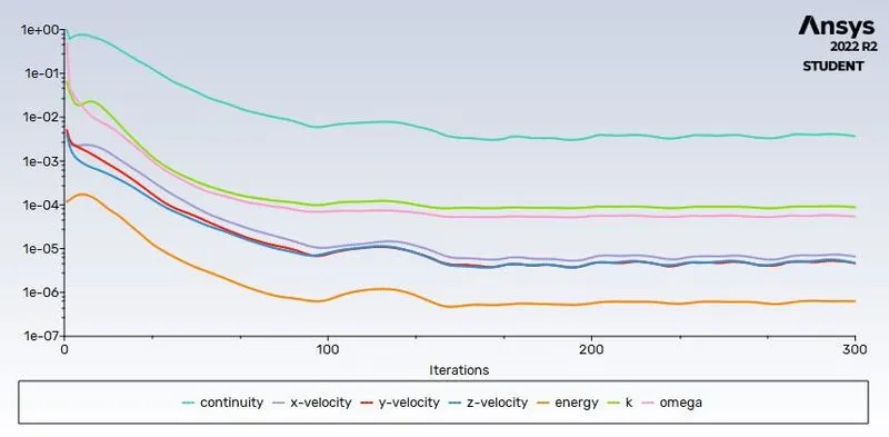
From the area weight average temp plot at the outlet, we can see that we get a converged value at 50 iterations.
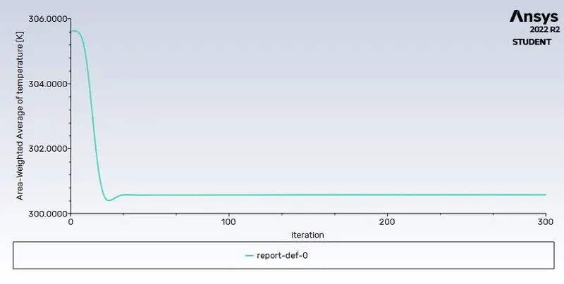
And form the standard deviation of temperature at the outlet we can say that the values of standard deviation have converged at about 80 iterations.
So now we will be post-processing our solution in CFD post.
In the CFD post, we will be creating a temperature contour at the midplane of the mixing Tee so we can see the temperature along and across the pipe.
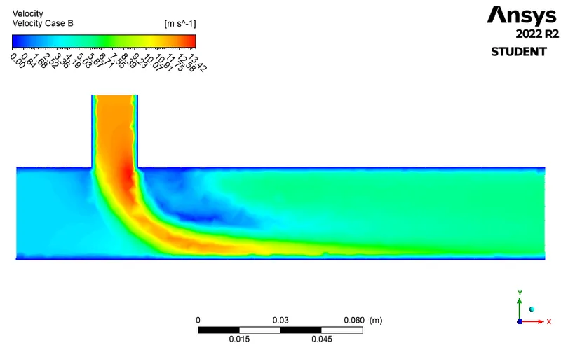
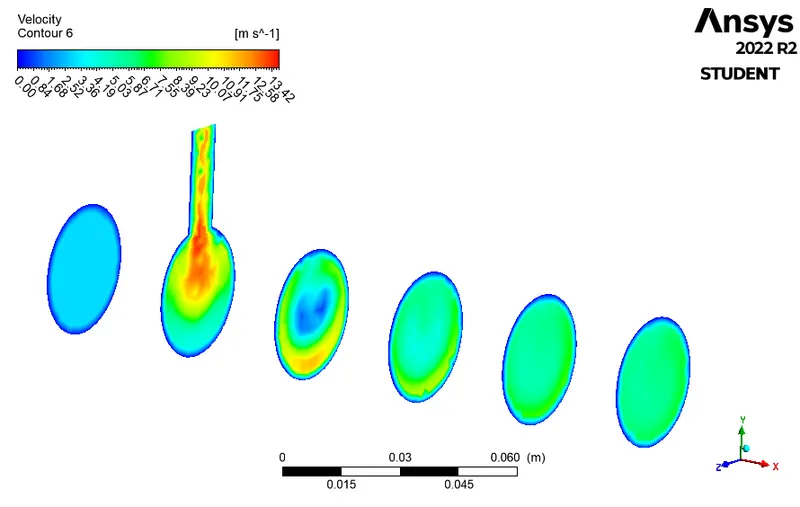
In the CFD post, we will be creating a Velocity contour at the midplane of the mixing Tee so we can see the temperature along and across the pipe.
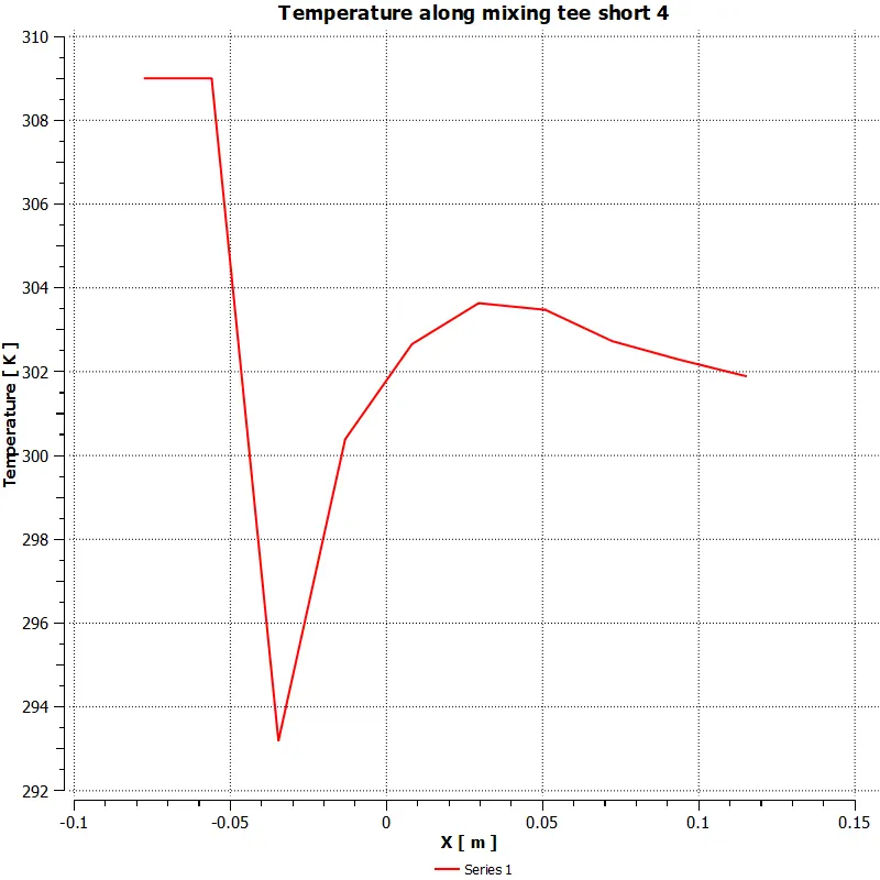
Various plots related to the solution are shown below:
Temperature plot along the pipe.
Velocity plot along the pipe.
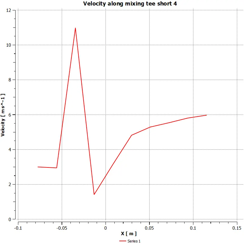
Table:
| Case Number | Momentum Ratio | Pipe Length | Average Temp Outlet |
No. of iterations for convergence |
| Case A | 2 | Short | 303.31 kelvin | 180 |
| Case B | 4 | Short | 300.58 kelvin | 210 |
| Case C | 2 | Long | 303.42 kelvin | 200 |
| Case D | 4 | Long | 300.50 kelvin | 280 |
Results:
The temperature contours show the mixing of hot and cold air flows.
For the short pipe length, the flow is not mixed properly
With increasing the length of the pipe the mixing of air increases and the standard deviation of temperature at the outlet is reduced
With standard deviation of temperature at the outlet also decreases when the cold inlet velocity is doubled.
We can find the best mixing in Case 2 (D), where due to the long length of the pipe and doubled cold inlet velocity the flow at the outlet is mixed properly and have a lower temperature.
By doubling the velocity of the cold inlet the temperature of the outlet decreases.
The plot of velocity and temperature along and across the pipe gives us an idea of how the flow distribution occurs at various positions in the pipe.
The velocity contours show how the turbulent flow along the length of the pipe and also we can see the boundary layer near the walls.
Finally, a Short mixing tee with a 3 mm mesh size, K-omega SST at moment ratio 4 produces the best results.
Conclusion:
Short mixing tee mesh size 3 mm with different momentum ratios 2, 4 respectively gives different Average outlet temperatures Momentum ratio (MR) = 2 gives more colling than MR = 4 because when MR = 2 cold inlet velocity is at 6 m/s whereas for MR = 4 cold inlet velocity is 12 m/s which double velocity as the first case. This shows that in case B higher velocity produces more turbulence in tee making better mixing of hot and cold air takes place to produce chilled air than case A. but case A converged more quickly than case B. Increase in momentum ratio produces better results. i.e., higher momentum ratios are recommended for better output.
The effect of length and momentum ratio on results.
In comparison to Cases 1 and 2 short, long mixing tee with the same mesh size and momentum ratios. The only difference is in the lengths of the pipes. long tee is 075.928 mm longer than the short tee. from this we can observe that an increase in the length of the pipe after a certain point does not produce major changes in results. from cases 1 and 2 an increase in length of 75.9 mm produced a temperature drop of 0.08 C which is negligible. Therefore short mixing tee is more suitable for this situation.
The effect of mesh size on results.
After comparing all three element sizes (1, 1.5, and 3 mm) it is found that as the element size is reduced the diffusion in the temperature contour reduces, and also there is a change in the values of the area-weighted temperature at the outlet. We get the best result with the smallest mesh size also we would have reduced the element size to 1 mm but the Ansys academic version does not support the number of elements generated by this size and exceed the limit. So we have to stop our grid test at 1.5 mm and we will be using the element size of 1.5 mm for the rest of the calculations for other cases with changing momentum ratio and the length of the mixing Tee.
The effect of the Viscous model on results.
When we compare the temperature and velocity plots from both K-epsilon and K-omega turbulence models for the same problem. where we used the same we can observe that K-omega captured more turbulence than K-epsilon. K epsilon is best suited for flow away from the wall, say free surface flow region, whereas the k-omega model is best suited for near the wall-flow region, where the adverse pressure gradient is developed. From the above calculations, we are going to use the K-omega SST turbulence model for further analysis.
Links:
1. Velocity Case 1(B) Short pipe Animation
https://drive.google.com/file/d/1e9F1SOHYHCOQGRAaJWdbt07bWBcvt9cC/view?usp=sharing
2. Temperature Case 1(B) Short pipe Animation
https://drive.google.com/file/d/12jUM-AWskQ1pHeOtzEoZEKZ-Mof5ioQL/view?usp=sharing