Week 1- Mixing Tee
Aim: To setup up steady-state simulations for the flow of air through mixing Tee in Ansys Fluent.
Objective:
1To set up the simulation for two cases i.e. Short and long mixing Tee.
2.To set up steady-state simulations to compare the mixing effectiveness when hot inlet temperature is 360C & the Cold inlet is at 190C.
3.To find out the average outlet temperature
4.Discuss the effect of length and momentum ratio on results.
Reference formula :-
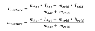
Introduction: In industrial process engineering, mixing is unit operation that involves the manipulation of heterogeneous physical system to make it more homogeneous. Modern industrial processing is always some form of mixing. Mixing Tee utilizes specifically engineered internal geometry to efficiently mix two fluid streams into single stream. Mixing Tee’s are widely used in the chemical and Refrigeration etc. industry in which fluid streams with different physical and chemical properties mixed together.
Theory:
k-omega SST:
The SST k-omega turbulence model is a two-equation eddy-viscosity model that is used for many aerodynamic applications. It is a hybrid model combining the Wilcox k-omega and the k-epsilon models. A blending function, F1, activates the Wilcox model near the wall and the k-epsilon model in the free stream. This ensures that the appropriate model is utilized throughout the flow field:
- The k-omega model is well suited for simulating flow in the viscous sub-layer.
- The k-epsilon model is ideal for predicting flow behavior in regions away from the wall.
- The SST models exhibit less sensitivity to free stream conditions (flow outside the boundary layer) than many other turbulence models.
- The shear stress limiter helps the k-omega model avoid a build-up of excessive turbulent kinetic energy near stagnation points.
k-epsilon:
K-epsilon (k-ε) turbulence model is the most common model used in Computational Fluid Dunamics (CFD) to simulate mean flow characteristics for turbulent flow conditions. It is a two equation model that gives a general description of turbulence by means of two transport equations (PDEs). The original impetus for the K-epsilon model was to improve the mixing length model as well as to find an alternative to algebraically prescribing turbulent length scales in moderate to high complexity flows.
- The first transported variable is the turbulent kinetic energy (k).
- The second transported variable is the rate of dissipation of turbulent kinetic energy (ε)
Procedure:
Geometry:
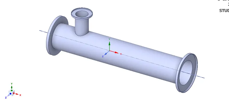
Geometry of Mixing is as follows:
Short tea :- For Case 1 and Case 2 short tea has been used as it is mentioned in the questions.
Long tea :-For case 2 and Case 3
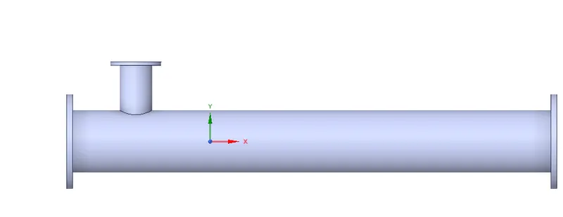
Case 1: short mixing tee with Momentum ratio 2
To simulate the mixing,we need to extract fluid volume. So spaceclaim we extracted the fluid volume from the geometry .
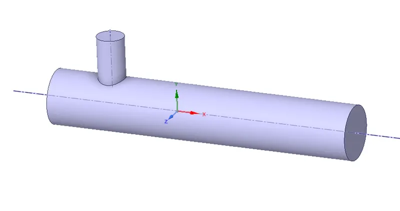
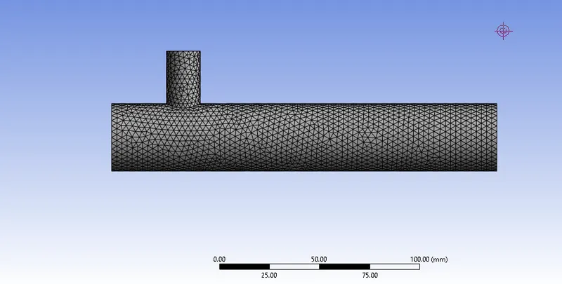
Then we meshed it using 3 mm as mesh length and set the named for inlet x ,inlet y, outlet and wall.
Mesh size - 3 mm
Number of nodes - 8369
Number of elements - 40039
Mesh quality criteria -
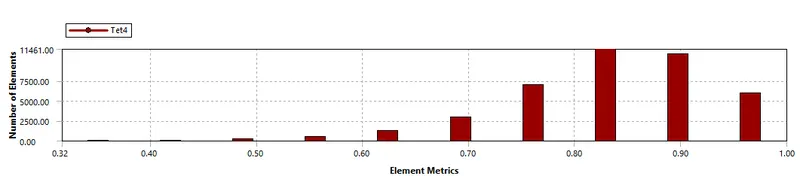
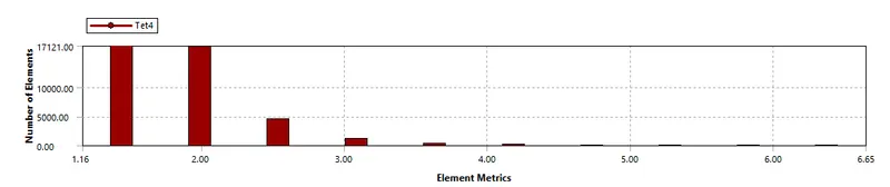
Majority of mesh elements are between 0.6 and 1 hence mesh quality is acceptable.
Then we have closed this mesh window and opened set up window by double clicked on it .
Setup:
1.Click on check mesh to know the mesh is acceptable or not.
2.To setup the flow physics, click on enery equation and as problem involves turbulence click on viscous > k-epsilon >relizable.
3. materials: air
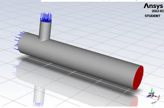
Boundary condition:
1.Inlet X
Velocity = 3 m/s
Temperature = 36 deg.C
2.Inlet Y
Velocity = 3*2 = 6 m/s
Temperature = 19 deg.C
3.Outlet
Gauge Pressure = 0 Pa
4.Wall
Velocity = No Slip
Solution:
1.Go to Solution > defination > select the parameters which we want to trace in ouput.
Here we want the magnitude of temperature and velocity, select area weighted average of temperature and velocity at outlet and also select standard deviation of temperature at outlet.
2.Hybrid initialization is done. Same will be shown in console.Hybrid inittialization process uses potential flow solver to compute an approximate value of velocity and pressure.
3.set the No. of iteration
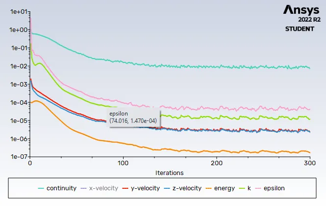
Residual plot:-
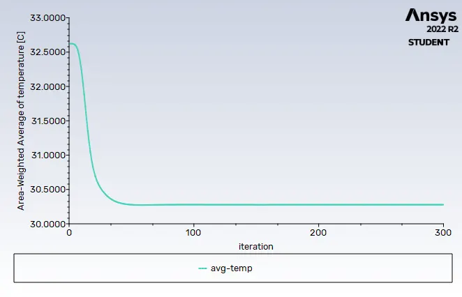
This problem has taken 175 iterations to converge.
Temperature :
Average outlet temperature is seems to be 30.35 C
Standard Deviation:
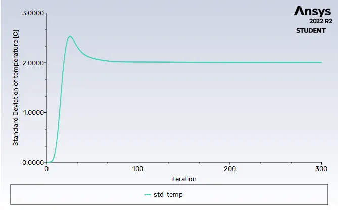
Here value of std of temp is showing 1.99
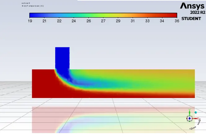
Temperature contour:
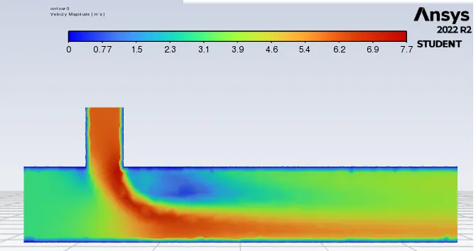
Velocity contour :
Case 2 :short mixing tee with Momentum ratio 4.
Foe Case 2 Geometry and mesh length are same as it is mentioned in question.
Boundary condition:
1.Inlet X
Velocity = 3 m/s
Temperature = 36 deg.C
2.Inlet Y
Velocity = 3*4 = 12 m/s
Temperature = 19 deg.C
3.Outlet
Gauge Pressure = 0 Pa
4.Wall
Velocity = No Slip
Solution:
1.Go to Solution > defination > select the parameters which we want to trace in ouput.
Here we want the magnitude of temperature and velocity, select area weighted average of temperature and velocity at outlet and also select standard deviation of temperature at outlet.
2.Hybrid initialization is done. Same will be shown in console.Hybrid inittialization process uses potential flow solver to compute an approximate value of velocity and pressure.
3.set the No. of iteration
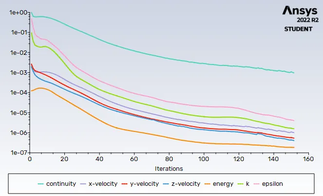
Residual plot:-
This problem has taken 152 iterations to converge.
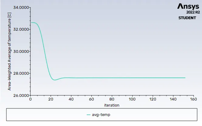
Temperature :
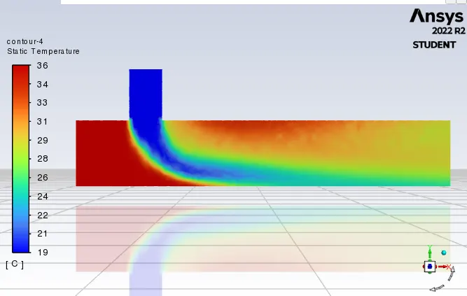
Average outlet temperature is seems to be 27.5 C
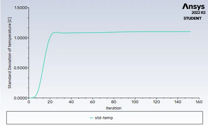
Standard Deviation:
Here value of std of temp is showing 1.99
Temperature contour:
velocity :
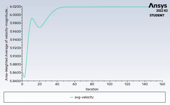
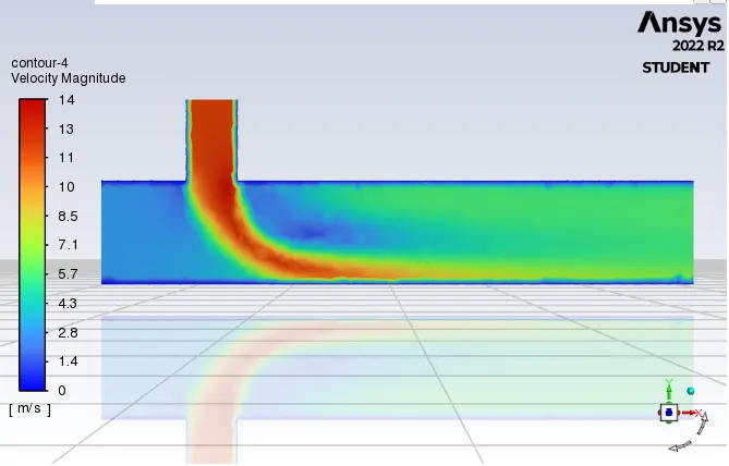
Average outlet velocity is seems to be 6.01m/s
Velocity contour:
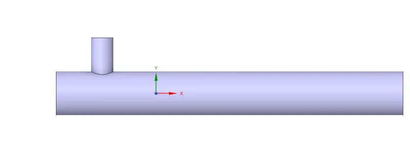
Case 3 :Long mixing tee with Momentum ratio 2
Afetr extracting the volume from the geometry
Then we meshed it using 3 mm as mesh length and set the named for inlet x ,inlet y, outlet and wall.
Mesh size - 3 mm
Number of nodes - 11766
Number of elements - 56884
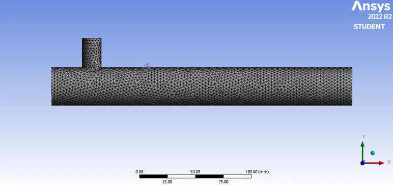
Mesh quality criteria :

Majority of mesh elements are between 0.6 and 1 hence mesh quality is acceptable.
Then we have closed this mesh window and opened set up window by double clicked on it .
Setup:
1.Click on check mesh to know the mesh is acceptable or not.
2.To setup the flow physics, click on enery equation and as problem involves turbulence click on viscous > k-epsilon >relizable.
3. materials: air
Boundary condition:
1.Inlet X
Velocity = 3 m/s
Temperature = 36 deg.C
2.Inlet Y
Velocity = 3*2 = 6 m/s
Temperature = 19 deg.C
3.Outlet
Gauge Pressure = 0 Pa
4.Wall
Velocity = No Slip
Solution:
1.Go to Solution > defination > select the parameters which we want to trace in ouput.
Here we want the magnitude of temperature and velocity, select area weighted average of temperature and velocity at outlet and also select standard deviation of temperature at outlet.
2.Hybrid initialization is done. Same will be shown in console.Hybrid inittialization process uses potential flow solver to compute an approximate value of velocity and pressure.
3.set the No. of iteration
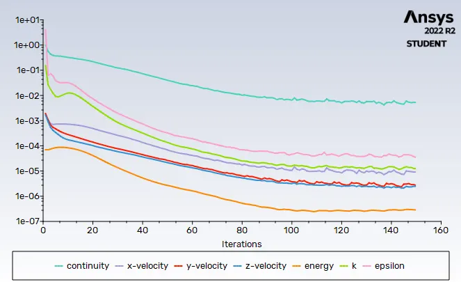
Residual plot:- This problem has taken 127 iterations to converge.
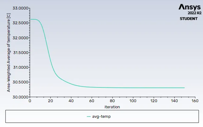
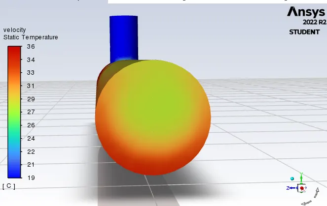
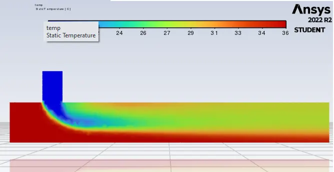
Temperature :Average outlet temperature is seems to be 30.35 C
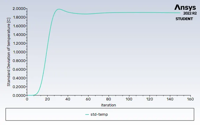
Temperature :Average outlet temperature is seems to be 1.99 C
Temperature contour :
velocity :
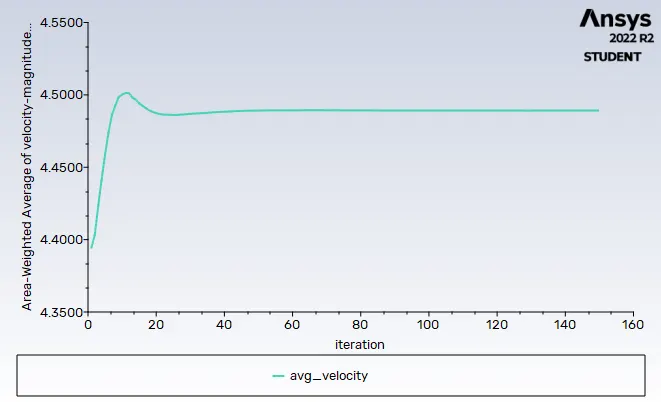
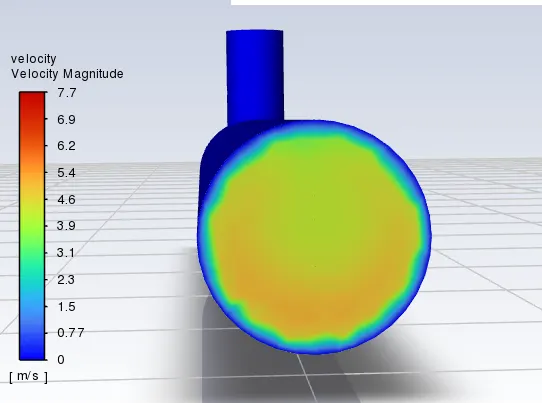
Average outlet velocity is seems to be 4.457 m/s
Velocity contour :
Case 4 :Long mixing tee with Momentum ratio 4.
Mesh:
Mesh length = 3 mm
Numner of nodes = 11766
Number of elements = 56884
Mesh quality : 
Boundary condition:
1.Inlet X
Velocity = 3 m/s
Temperature = 36 deg.C
2.Inlet Y
Velocity = 3*4 = 12 m/s
Temperature = 19 deg.C
3.Outlet
Gauge Pressure = 0 Pa
4.Wall
Velocity = No Slip
Solution:
1.Go to Solution > defination > select the parameters which we want to trace in ouput.
Here we want the magnitude of temperature and velocity, select area weighted average of temperature and velocity at outlet and also select standard deviation of temperature at outlet.
2.Hybrid initialization is done. Same will be shown in console.Hybrid inittialization process uses potential flow solver to compute an approximate value of velocity and pressure.
3.set the No. of iteration
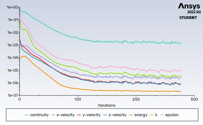
Residual plot:- This problem has taken 185 iterations to converge.
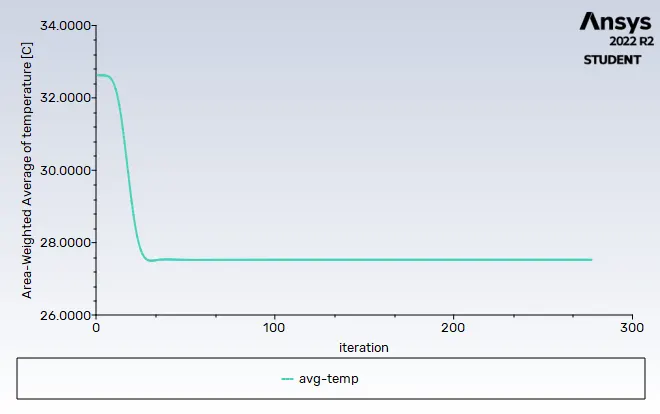
Temperature :Average outlet temperature is seems to be 27.5 C
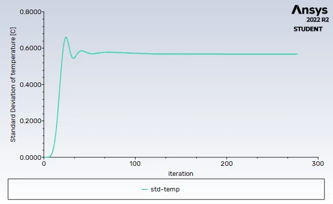
Std plot of temperature : 0.58 degree.C
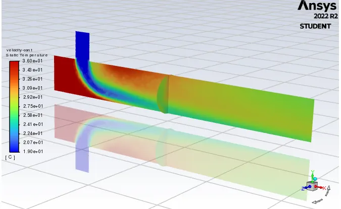
Temperature contour :
velocity :
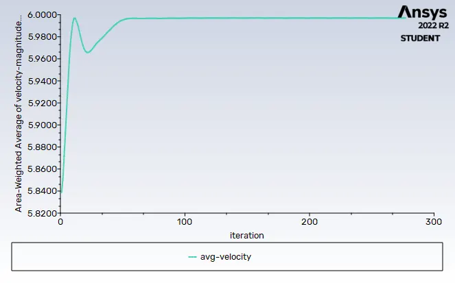
Average outlet velocity is seems to be 5.99 m/s
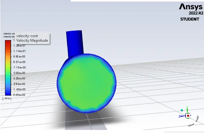
Velocity contour :
Effect of turbulence model
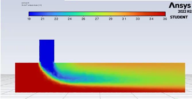
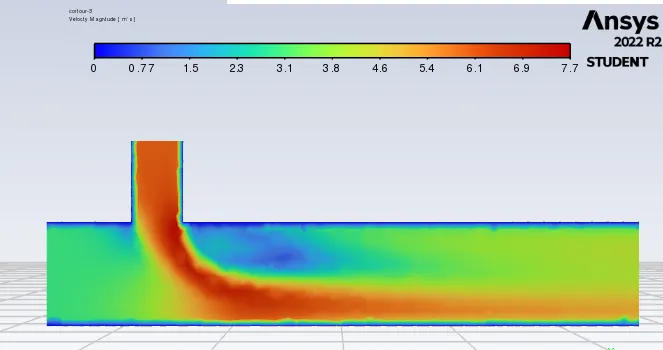
Here we are taking case of short mixing tee with momentum ratio of 2 and run it using k-epsilon same as Case 1 number and k-omega SST model to detrmine the effect of turbulence model on output.
We have already completed short mixing tea with MR 2 and tun it using K -epsilon . Now we will duplicate case 1 and perform set up , solution, result again using k -omega sst model to determine the effect of turbulence model .
Mesh -
Mesh length = 3mm
Number of nodes = 8369
Number of elements = 40039
Mesh quality criteria :
Boundary condition:
1.Inlet X
Velocity = 3 m/s
Temperature = 36 deg.C
2.Inlet Y
Velocity = 3*2 = 6 m/s
Temperature = 19 deg.C
3.Outlet
Gauge Pressure = 0 Pa
4.Wall
Velocity = No Slip
Solution:
1.Go to Solution > defination > select the parameters which we want to trace in ouput.
Here we want the magnitude of temperature and velocity, select area weighted average of temperature and velocity at outlet and also select standard deviation of temperature at outlet.
2.Hybrid initialization is done. Same will be shown in console.Hybrid inittialization process uses potential flow solver to compute an approximate value of velocity and pressure.
3.set the No. of iteration
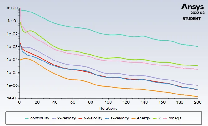
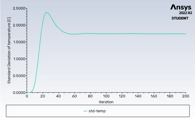
Residual plot:- This problem has taken 200 iterations to converge.
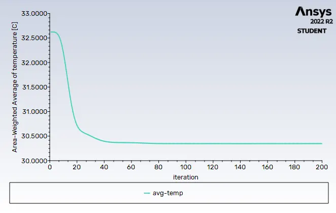
Temperature :Average outlet temperature is seems to be 30.35 degree C
Std plot of temperature :
Temperature contour :
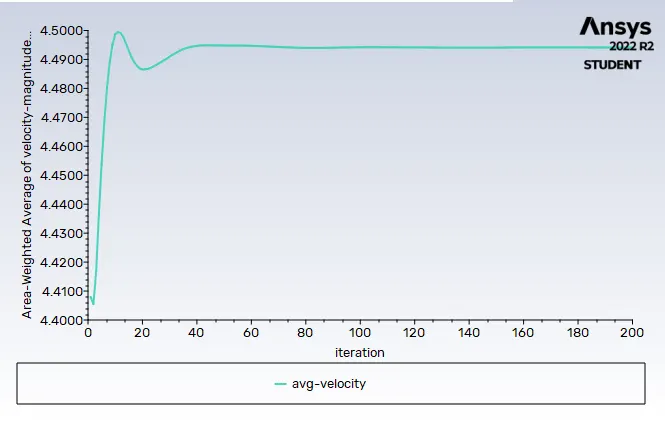
Temperature :Average outlet velocity is seems to be 4.46 m/s
Temperature contour :
Result Discussion:
Effect of Turbulence model:

Effect of Momentum Ratio :
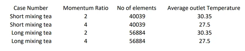
Conclusion/ Observation :-
1.k-epsilon predicts well far from boundaries and k-omega model predicts well near the boundary,as in this case we are not dealing with walls, we have used k-epsilon model for further simulation.
2.Momentum ratio is the ratio of velocity at cold inlet to velocity at hot inlet.From the above plot we can understand that tha increasing the velocity of cold inlet with respect to velocity of hot inlet by factor of momentum ratio gives better mixing of hot and cold fluid stream at outlet.
3.Standard deviation of temperature is defference in temperature value outlet as compared to average temperature value.from the plots of standard deviation of temperature,it is observed that standard deviation of temperature is minimum for the case of long mixing tee with momentum ratio.
Effect of length:-
As from the above results, it can be inferred that length has no effect on average temperature at the outlet.
Therefore short mixing tee should be preferred.
Effect of momentum ratio:-
Results show a significant effect of momentum ratio on outlet temperature. As the temperature is decreasing with an increase in momentum ratio. From the temperature contour, it can also be seen that mixing is largely influenced by momentum ratio (inlet velocity of cold stream).