Week 1- Mixing Tee

Aim:

• To set up steady-state simulations to compare the mixing effectiveness when the hot inlet temperature is 36 C, and the cold inlet is 19 C.
• To compare the k-epsilon and k-omega SST models for the first case to get proper judgment about each method.
• Simulate each case for the given velocity and momentum ratio.
• Compare results from the 2 cases about cell count, average outlet temperature, and the number of iterations for convergence.

Objective:

• Open Ansys workbench and set up a fluent simulation setup, and rename it accordingly.
• Open space claims, a fluid setup, and loading the geometry.
• Identify the working fluid region in the loaded geometry and run the simulation there. Close the space claim after that.
• Next, specify boundary names for each surface in the mesh setup before creating a mesh for the fluid flow volume. Update the mesh after closing the mesh setup.
• Provide all the necessary parameters for the simulation in the setup section later on, including the simulation type, input velocity and temperature, materials (working fluid), and other user-defined parameters.
• Learn about the k-epsilon and k-omega SST concepts in setup parameters and determine which is best for the current simulation.
• After that, simulate our problem setup to determine how many iterations are necessary for our results to converge.
• Close the setup after that and update it. To view, all of the simulated results, open the results section.
• Results for each case's cell count, average outlet temperature, and convergence iteration count were generated by Combine.
• Study the effect of length and momentum ratio on the results of each case.

Introduction:

• Computational fluid dynamics is a branch of fluid mechanics, which uses mathematics, physics and computational software to visualize how fluid flows and affects its medium and its neighbours. In CFD mostly computers are used to predict the fluid flow phenomena based on some governing equations like conservation of momentum – Navier stokes equation, conservation of energy etc. In this study, we are going to simulate the effect of fluid using Ansys fluent software. Ansys fluent is a very important tool in the CAE domain, which allows you to perform all three major steps of any simulation pre-processing, solving and post-processing. Ansys fluent facilitates for modelling flow, turbulence, heat transfer and chemical reactions. With Ansys, we can accomplice more in less time and with less training.
• Mixing tee is a device which uses specifically engineered internal geometry to mix two fluid streams into one steam, efficiently. In this study, we are going to find the effectiveness of mixing tee. Hot air and cold air are going to be mixed in a mixing tee. They will have different velocities. We will use two different mixing tees distinguished with length and analyse the effect of length on mixing.

Primary Conditions:

Understand k-epsilon and k-omega SST by considering case-1

Case-1;

• Short mixing tee

a - Simulation-1

hot Inlet velocity - 3 m/s

Momentum ratio - 4

b - Simulation-2

hot Inlet velocity - 3 m/s

Momentum ratio - 2

Case-2;

• Long mixing tee

a - Simulation-3

hot Inlet velocity - 3 m/s

Momentum ratio - 4

b - Simulation-4

hot Inlet velocity - 3m/s

Momentum ratio - 2

where Momentum ratio = velocity at cold inlet/velocity at hot inlet.

Procedure:

• The first study will set two setups, one for k-epsilon and another for k-omega SST. Here, we are going to use the same geometry and mesh for both cases of simulation. Hence, we are going to use a short mixing tee model and mesh it.

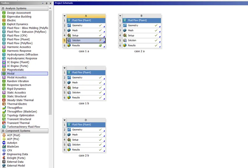
• Now click on geometry to import mixing tee model. It will redirect to Spaceclaim, Ansys’s geometry model manipulator.
• Then open space claim to load geometry in setup. Space claim is a beneficial CAD cleanup software to prepare CAD geometry for simulation setup; it could be for FEA or CFD.

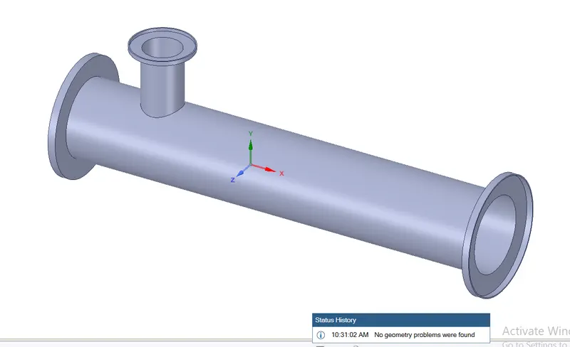
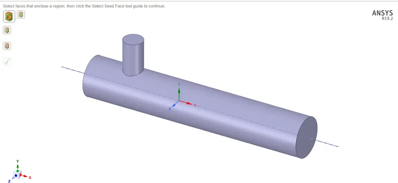
• We are to analyse the mixing of two fluids, so there is a role of parts other than two pipes. To suppress that we need to extract the volume of a tee. Go to prepare the menu and click on volume extract. Switch to edge selection and select three outer edges and click on the green check button.

• Hide solid by unchecking it from the structure menu to see the volume, which we have extracted.

• Suppress solid by clicking on the option suppress for physics.

• Exit from Spaceclaim and click on the mesh to open the mesh menu.

• Select an outer face and press the right click of a mouse, it will open a menu. Click on the option to create a named selection and write a suitable name for the face. Repeat for other faces.

• Now, we can go for meshing. So, click on the mesh button, which will start Ansys meshing, where we can generate the mesh and provide names for all the surfaces of the geometry.

• Next, create two fluent setups—one for k-epsilon and another for k-omega SST. Drag the exiting mesh into the Fluent analysis Setup cell. Then update the mesh (Right-click on mesh and use the update button) to convert and write the mesh for the FLUENT analysis.

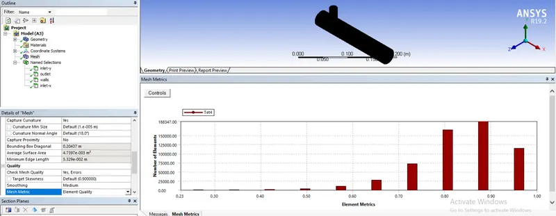
• And we can also investigate the quality of mesh by clicking on the option called element quality in the quality section of the mesh panel.
• Then, double-click on the setup option in the FLUENT cell for trying the k-epsilon method. It will open the FLUENT interface.
• In the Fluent window, we will first see the console window which displays text, and also accepts TUI (Text User Interface) commands. In the beginning, we will see a lot of text about loading meshing cells, and text about achromatic setting boundary conditions in fluent as per the name provided to surfaces.
• After clicking on the check mesh quality button, it prints the following conformation in the Console Window. The mesh check ensures that each cell is in the correct format and connected to other cells as expected. It is recommended to check every mesh immediately after reading it. Failure of any check indicates a badly formed or corrupted mesh that will need repairs prior to simulation.

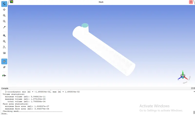
• Next, in the domain panel by using the check button we can check whether our mesh is preferable for fluent analysis or not. And we can improve the quality using modify option.

• Click ‘units’ to change the units of temperature. FLUENT store values in SI units. Most post-processing can be converted into other units.
• Then we will set the physics of the domain. Keep the general parameter setting as it is. Solver type -> pressure-based; velocity formulation -> Absolute; solver time -> steady.

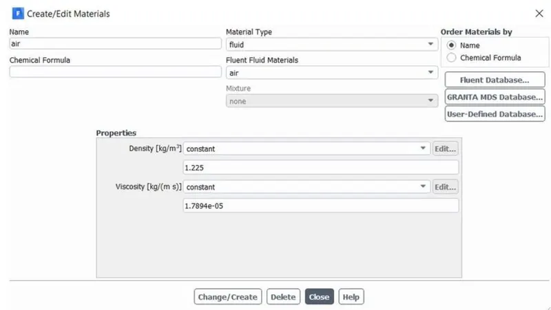
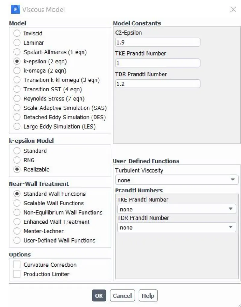
• Go to the physics menu and select a viscous model. It will open a menu, choose a realizable k-epsilon model and close it.
• In materials click “FLUENT Database’ to add new material. In this case, our working fluid is air so we keep the default material.
• In the viscus model, select ‘k-epsilon’, and’ Realizable’ for our first type of simulation. Turbulence modelling is a complex area. The choice of model depends on the application. Here, the Realizable k-epsilon model is used which is an improvement on the well-established standard k-epsilon model. Accept the remaining default settings.

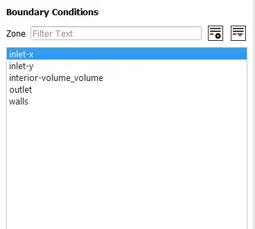
• Now go to the boundaries option to set boundary conditions. Select inlet_x and click on the option edit. It will open a menu, where all the parameters can be set whether it is thermal, radiation, momentum etc. Put the value of velocity as 3 m/s and go to the thermal parameter to set the temperature as 36 C, for hot fluid.

• And, a similar way creates a plot for average velocity plot at outlet boundary condition.

• Before running the program our final step will be to initialize the problem setup.

• Initialization creates the initial solution that the solver will iteratively improve. Generally, the same converged solution is reached whatever the initialization, though convergence is easier if they are similar. Basic initialization imposes the same values in all cells. You can improve on this in various ways - for example, by patching different values into different zones. Several features, including patching and post-processing, are not available until after initialization.

• The hybrid Initialization method is an efficient method of initializing the solution based purely on the setup of the simulation with no extra information required. These methods produce a velocity field that conforms to complex domain geometries and a pressure field that conforms to complex domain geometries and a pressure field that smoothly connects high and low-pressure values.

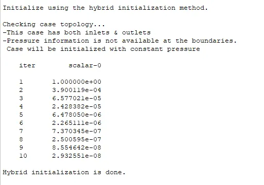
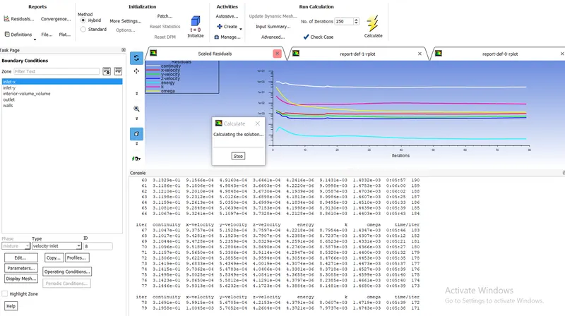
• Now, we can run the simulation just enter the number of iterations for which we want to run the simulation and press ‘calculate’.

• Repeat the same procedure for cold fluid coming, velocity – 6 m/s, temperature – 19C.

• We want to generate a temperature report of the outlet and we want a standard deviation of temperature also.

• Go to the Solutions tab and select definition and select area-weighted average. In the opened menu select temperature as the field variable. Similarly, select standard deviation in the definitions menu.

• Now click on initialization to calculate approximate values of velocity and pressure. Change the number of iterations to 250 and click on calculate. If a solution is not converged, then iterations can be increased.

• Exit setup and double-click on the result to open the CFD post. Checkboxes to see walls and other parts.

• CFD-Post initially displays the outline (wireframe) of the model which can be turned on by checking the surface shown in the Outline panel in the fluid section.

• Viewer toolbar buttons allow you to manipulate the view.

• Create a plane - in the location menu, select ‘Plane’ -> accept the default name ‘Plane 1’ -> set ‘Method’ to be ‘XY Plane, accept ‘Z’ as 0.0, and press ‘Apply’

• k-Epsilon: As we saw in our first simulation, the K-epsilon turbulence model is the most common model used in CFD to simulate mean flow characteristics for turbulent flow conditions. It is a two-equation model that gives a description of turbulence by means of two transport equations (PDEs). the first transported variables are the turbulent kinetic energy (k) and the second transported variable is the rate of dissipation of turbulent kinetic energy. k-epsilon focuses on the mechanism that affects the turbulent kinetic energy.

• k-omega SST: The SST k-omega turbulence model is a two-equation eddy-viscosity model that is used for many aerodynamic applications. It is a hybrid model combining the Wilcox k-omega and the k-epsilon models. A blending function, F1, activates the Wilcox model near the wall and the k-epsilon model in the free stream. This ensures that the appropriate model is utilized through the flow field.

Results:

• The viscous sub-layer flow can be accurately simulated using the k- omega model. The k-epsilon model, however, is superior for predicting flow in areas far from the wall. Compared to many other turbulence models, the SST model is less sensitive to free stream conditions (Flow outside the boundary layer).

• The k-omega model is assisted by the shear stress limiter in preventing an accumulation of excessive turbulent kinetic energy close to stagnation points. If we look at our simulation figure, we can see that the k-omega model's flow is more laminar and does not produce proper turbulent results, while the k-epsilon model's simulation produces proper mixing of the two air streams. Since walls are not involved in this particular situation, we will use the k-epsilon method for further simulations.

Now, let us start our simulation with case 1 - a,

1.Case-1-a (Short mixing tee):

• a - Simulation-1,
• Inlet velocity - 3m/s,
• Momentum ratio - 4,
• Inlet velocity of cold air = 3x4 = 12m/s.

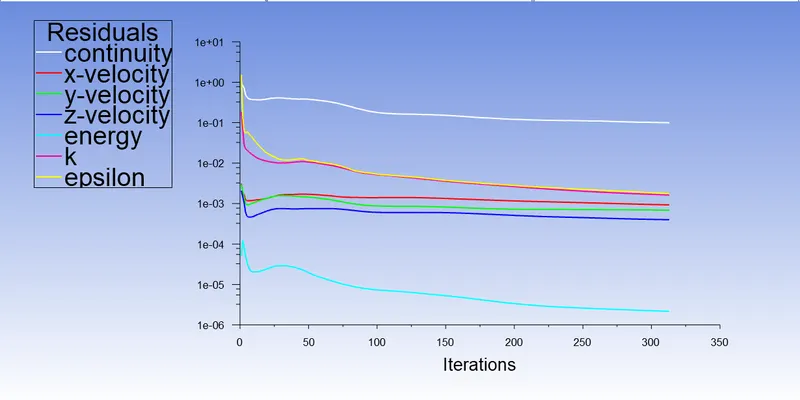
• Residue plot:

The solution is converging at 325 iterations.

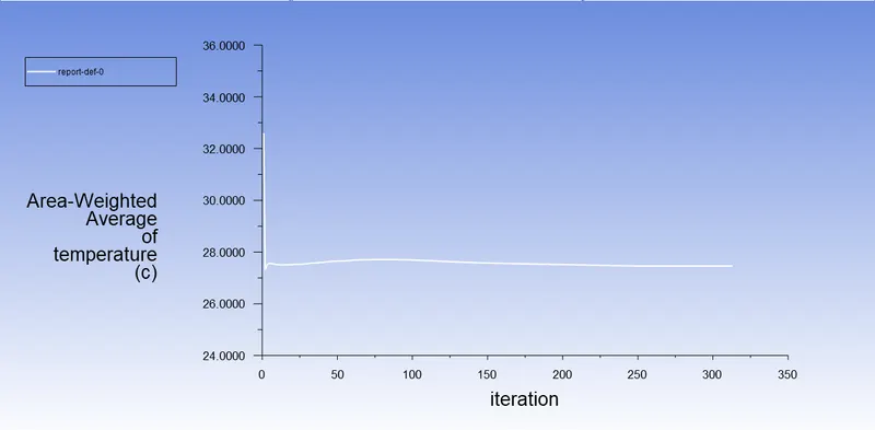
• Average Temperature vs Iterations:

Area weighted average outlet temperature:

The average temperature at the outlet is 27.78^oC.

• Standard Deviation of Temperature vs Iteration:

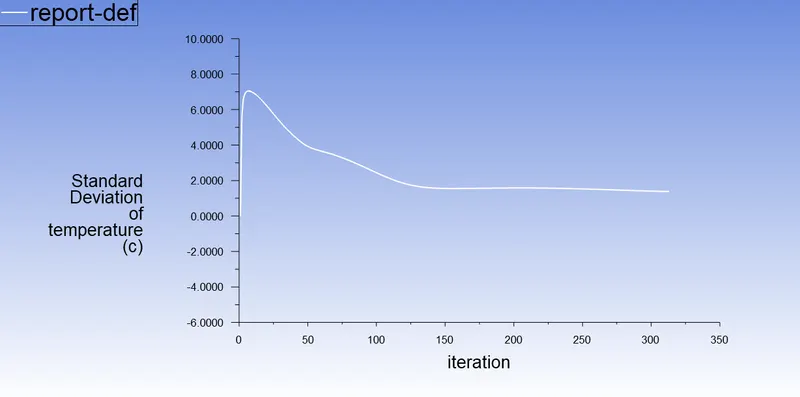
• Temperature contour on the plane along the length of the pipe:

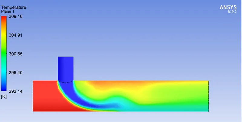
• Temperature Streamline on the plane along the length of the pipe:

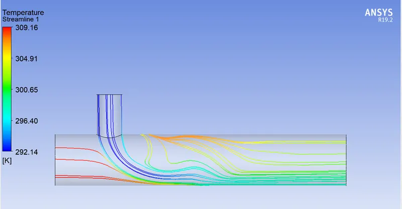
• Velocity contour on the plane along the length of pipe:

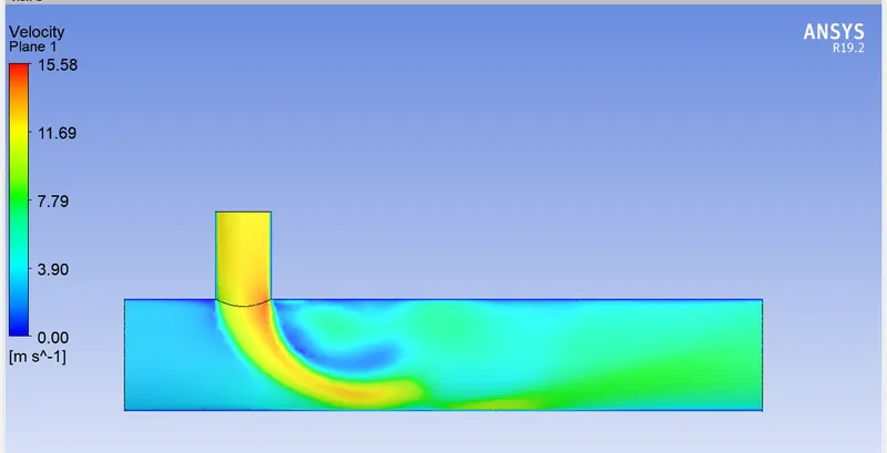
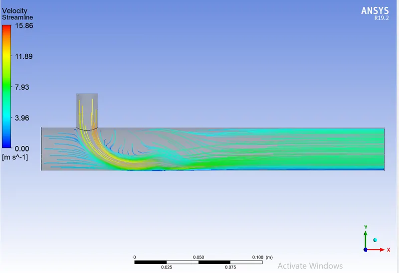
• Velocity Streamline on the plane along the length of the pipe:

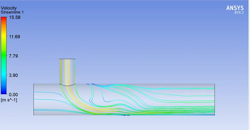
2. Case-1-b (Short mixing tee):

• b - Simulation-1,
• Inlet velocity - 3m/s,
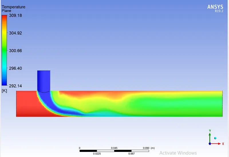
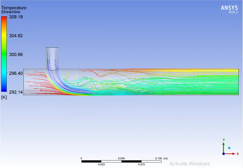
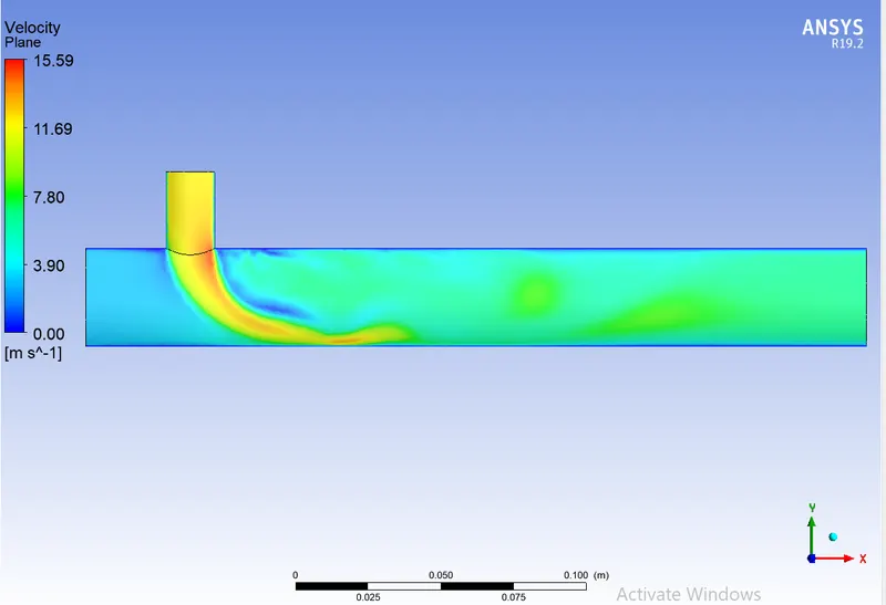
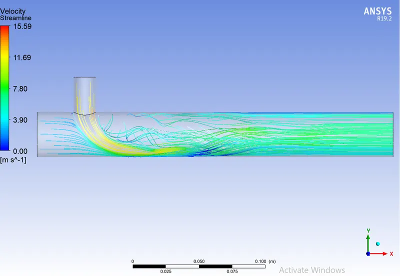
• Momentum ratio - 2,
• Inlet velocity of cold air = 3x2 = 6m/s.

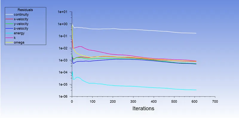
• Residue plot:

The solution is converging at 613 iterations.

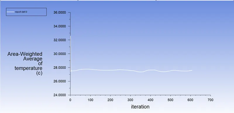
• Average Temperature vs Iterations:

Area weighted average outlet temperature:

The average temperature at the outlet is 27.67^oC.

• Standard Deviation of Temperature vs Iteration:

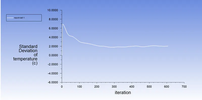
• Temperature contour on the plane along the length of the pipe:

• Temperature Streamline on the plane along the length of the pipe:

• Velocity contour on the plane along the length of pipe:

• Velocity Streamline on the plane along the length of the pipe:

3.Case-2-a (Long mixing tee):

• a - Simulation-1,
• Hot Inlet velocity - 3m/s,
• Momentum ratio - 4,
• Inlet velocity of cold air = 3x4 = 12m/s.

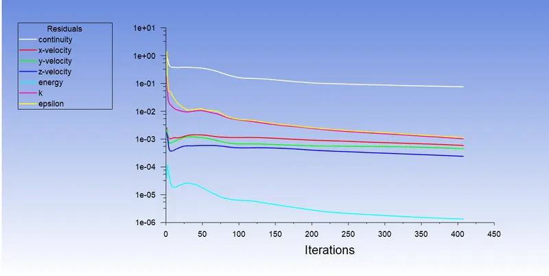
• Residue plot:

The solution is converging at 417 iterations.

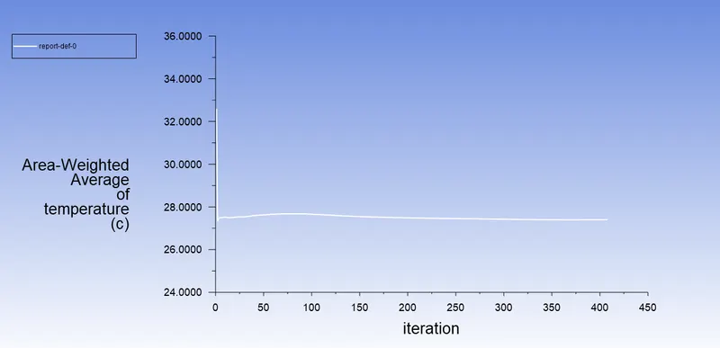
• Average Temperature vs Iterations:

Area weighted average outlet temperature:

The average temperature at the outlet is 28.56^oC.

• Standard Deviation of Temperature vs Iteration:

• Temperature contour on the plane along the length of the pipe:

• Temperature Streamline on the plane along the length of the pipe:

• Velocity contour on the plane along the length of pipe:

• Velocity Streamline on the plane along the length of the pipe:

4.Case-2-b (long mixing tee):

• b - Simulation-1,
• Inlet velocity - 3m/s,
• Momentum ratio - 2,
• Inlet velocity of cold air = 3x2 = 6m/s.

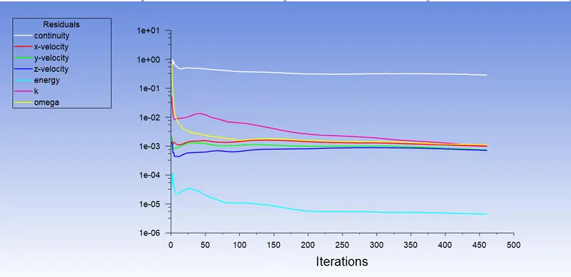
• Residue plot:

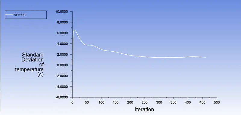
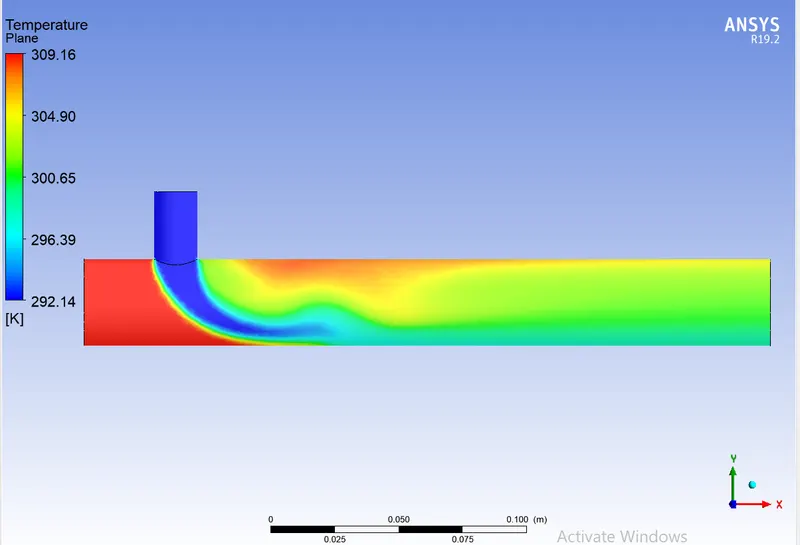
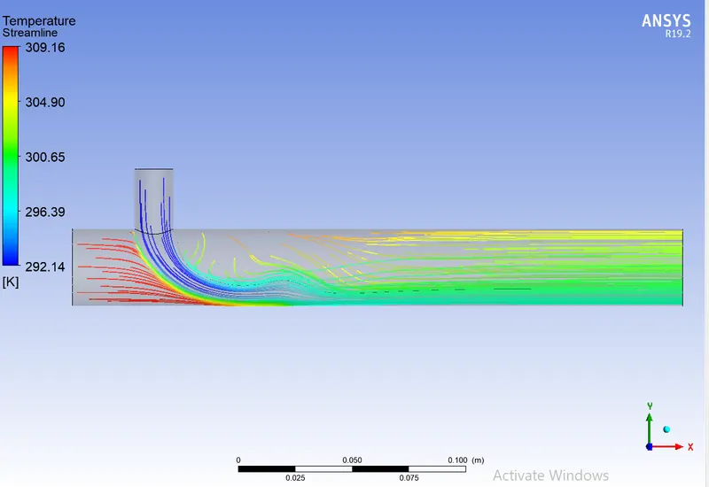
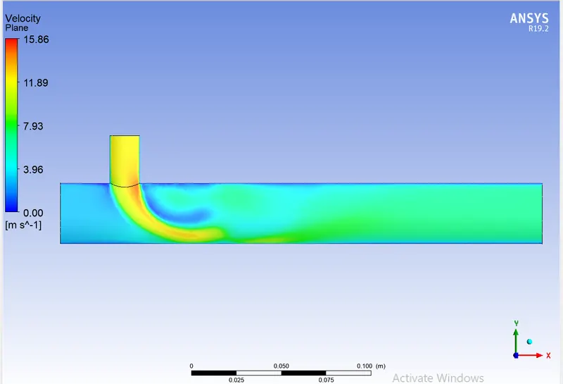
The solution is converging at 465 iterations.

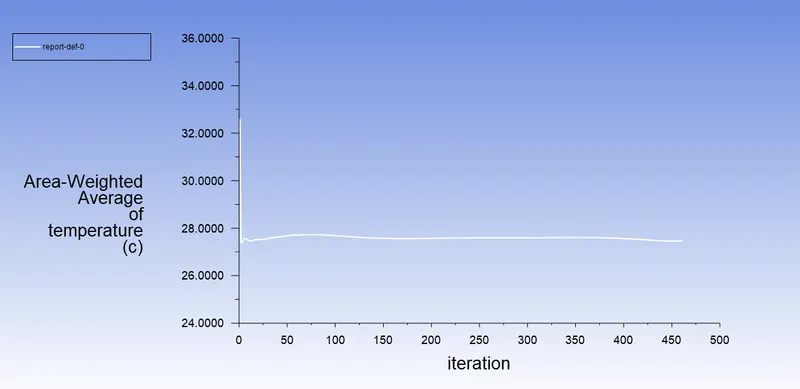
• Average Temperature vs Iterations:

Area weighted average outlet temperature:

The average temperature at the outlet is 27.87^oC.

• Standard Deviation of Temperature vs Iteration:

• Temperature contour on the plane along the length of the pipe:

• Temperature Streamline on the plane along the length of the pipe:

• Velocity contour on the plane along the length of pipe:

• Velocity Streamline on the plane along the length of the pipe:

Conclusion:

• Solving the first simulation on the fluid domain using coarse mesh gives an initial overview of the analysis which converges results fast. As the element number increases the convergence time also increases. Therefore, after obtaining the rough results using coarse mesh simulation successfully we can improve mesh quality and get to final accurate results doing this saves a lot of time which is also extremely helpful for the mesh independence tests.
• To get better mixing at outlet high velocity of flow is very effective. Therefore, a higher momentum ratio gives better mixing of hot and cold fluid streams at the outlet.
• The Cell count for cases 1- 12657 and for cases 2 - 15675.
• As the Length of the mixing tee increases because diffusion flow always gives slightly better mixing of two-fluid.
• In this study, we performed simulation on simple geometry of mixing tee and got insights of various features of fluent. we can conclude by analysing the graph that If the momentum ratio is increased, outlet temperature will decrease and there is no effect of velocity even though the length is increased.
• To obtain accurate results, it is crucial to use a short mixing tee with a momentum ratio of 4. However, one must take into account the diffusion of flow along the length of the mixing tee; in this case, a long mixing tee with momentum would be preferable.

Reference:

• https://www.sciencedirect.com/science/article/abs/pii/S0029549309005676