Week 5 - Genetic Algorithm

Aim:

• To write code in MATLAB to optimize the stalagmite function and find the global maxima of the function.

Objective:

• Explanation of the concept of a genetic algorithm (ga),
• Explanation of syntax for ga in MATLAB.

FACTORS ENTAILED:

Genetic algorithm:

• A genetic algorithm (or GA) is a search technique used in computing to find true or approximate solutions to optimization and search problems.
• (GA)s are categorized as global search heuristics.
• (GA)s are a particular class of evolutionary algorithms that use techniques inspired by evolutionary biologies such as inheritance, mutation, selection, and crossover (also called recombination).

GA Operators and Parameters:

• Selection
• Crossover
• Mutation.

Selection:

• The process determines which solutions are to be preserved and allowed to reproduce and which ones deserve to die out. The primary objective of the selection operator is to emphasize the good solutions and eliminate the bad solutions in a population while keeping the population size constant.
• Functions of the Selection operator, Identify the good solutions in a population Make multiple copies of the good solutions, and Eliminate bad solutions from the population so that multiple copies of good solutions can be placed in the population.

Crossover operator:

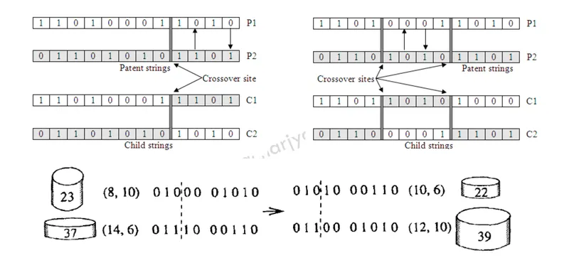
• The most popular crossover selects any two solutions strings randomly from the mating pool and some portion of the strings is exchanged between strings.
• The selection point is selected randomly.
• A probability of crossover is also introduced in order to give freedom to an individual solution string to determine whether the solution would go for crossover or not.

Binary Crossover:

Mutation operator:

• The mutation is the occasional introduction of new features into the solution strings of the population pool to maintain diversity in the population.
• Though crossover has the main responsibility to search for the optimal solution, the mutation is also used for this purpose.

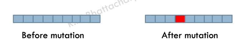
Binary Mutation:

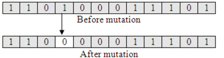
• The mutation operator changes a 1 to 0 or vice versa, with a mutation probability of.
• The mutation probability is generally kept low for steady convergence.
• A high value of mutation probability would search here and there like a random search technique.

NOTE :

• A genetic Algorithm is only used to generate a minimum solution. So the value of the stalagmite function is taken negatively to maximise the function.

Matlab Program:

• STALAGMITE FUNCTION:

Initially, we will start our code with all the input parameters and define a function into another 'stalagmite(input_vector)'

function [f] = stalagmite(input_vector)
f1x = (sin((5.1*pi).*input_vector(1)+0.5)).^6;
f1y = (sin((5.1*pi).*input_vector(2)+0.5)).^6;

f2x = exp((((input_vector(1)-0.0667).^2)/0.64).*(-4*log(2)));
f2y = exp((((input_vector(2)-0.0667).^2)/0.64).*(-4*log(2)));
f1=f1x*f1y*f2x*f2y;
f=-f1;

Evaluating the stalagmite function:

• The code is written to check if the function is returning an output.
• The function creates a 3D plot showing the Algorithm.

clear all 
close all
clc

n=150;
x = linspace(0,0.6,150);
y = linspace(0,0.6,150);

tic

%creating the two-dimensional grid
[xx, yy] = meshgrid(x,y);

%evaluating the stalagmite function

for i = 1:length(xx)
    for j = 1:length(yy)
        input_vector(1)= xx(i,j);
        input_vector(2)= yy(i,j);
        f(i,j) = stalagmite(input_vector);
    end
end

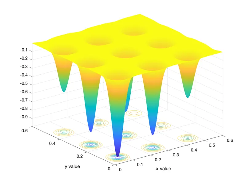
figure(1)
surfc(xx, yy, f)
shading interp
xlabel('x value');
ylabel('y value');
study_time=toc;

• Case-1 (Unbounded Inputs):

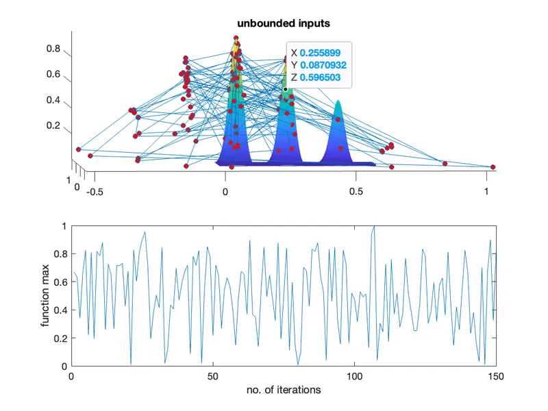
For the Unbounded Stalagmites, the code starts with a ‘tic’ having the inputs and optimal function with calling the function.The plot is generated with unbounded stalagmites

tic

for i = 1:n
    [inputs,fopt(i)]= ga(@stalagmite, 2);
    xopt(i)=inputs(1);
    yopt(i)=inputs(2);
end

figure(2)
subplot(2,1,1)

hold on
surfc (x,y,-f)
shading interp

plot3(xopt,yopt,-fopt,'marker','o','markersize',5,'markerfacecolor','r')
title('unbounded inputs')

subplot(2,1,2)
plot(-fopt)

xlabel('no. of iterations');
ylabel('function max');

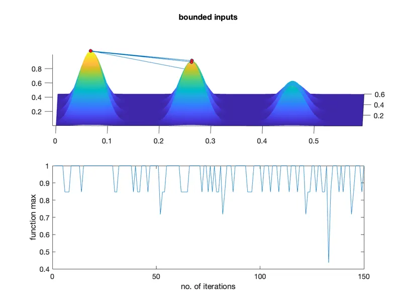
study_time1=toc;

• Case-2 (Bounded Inputs):

The code is written for the genetic algorithm function built-in inside the MATLAB. An empty array is created with starting and ending points of the x and y values.The plot is created with the inputs in the proper order.

tic

for i = 1:n
    [inputs,fopt(i)]= ga(@stalagmite, 2,[],[],[],[],[0;0],[0.6;0.6]);
    xopt(i)=inputs(1);
    yopt(i)=inputs(2);
end

figure(3)
subplot(2,1,1)

hold on

surfc (x,y,-f)
shading interp

plot3(xopt,yopt,-fopt,'marker','o','markersize',5,'markerfacecolor','r')

title('bounded inputs')
subplot(2,1,2)

plot(-fopt)

xlabel('no. of iterations');
ylabel('function max');

study_time2=toc;

• Case-3 (Bounded Inputs with increased population size):

• The code begins with writing ‘optimoptions’. The details are given in the ‘Factors Entailed’
• The plot is then created as the previous method.

tic

options=optimoptions('ga');
options=optimoptions(options,'PopulationSize',500);

for i = 1:n
    [inputs,fopt(i)]= ga(@stalagmite,2,[],[],[],[],[0;0],[1;1],[],[],options);
    xopt(i)=inputs(1);
    yopt(i)=inputs(2);
end

figure(4)

subplot(2,1,1)

hold on

surfc (x,y,-f)
shading interp
plot3(xopt,yopt,-fopt,'marker','o','markersize',5,'markerfacecolor','r')

title('bounded inputs with increases population')
subplot(2,1,2)
plot(-fopt)

xlabel('no. of iterations');
ylabel('function max');

study_time3=toc;

MAIN CODE:

For Function:

function [f] = stalagmite(input_vector)
f1x = (sin((5.1*pi).*input_vector(1)+0.5)).^6;
f1y = (sin((5.1*pi).*input_vector(2)+0.5)).^6;

f2x = exp((((input_vector(1)-0.0667).^2)/0.64).*(-4*log(2)));
f2y = exp((((input_vector(2)-0.0667).^2)/0.64).*(-4*log(2)));
f1=f1x*f1y*f2x*f2y;
f=-f1;

For Main Function:

clear all 
close all
clc

n=150;
x = linspace(0,0.6,150);
y = linspace(0,0.6,150);

tic

%creating two dimensional grid
[xx, yy] = meshgrid(x,y);

%evaluating the stalagmite function

for i = 1:length(xx)
    for j = 1:length(yy)
        input_vector(1)= xx(i,j);
        input_vector(2)= yy(i,j);
        f(i,j) = stalagmite(input_vector);
    end
end

figure(1)
surfc(xx, yy, f)
shading interp
xlabel('x value');
ylabel('y value');
study_time=toc;

%case 1 (unbounded inputs)

tic
for i = 1:n
    [inputs,fopt(i)]= ga(@stalagmite, 2);
    xopt(i)=inputs(1);
    yopt(i)=inputs(2);
end

figure(2)
subplot(2,1,1)
hold on
surfc (x,y,-f)
shading interp
plot3(xopt,yopt,-fopt,'marker','o','markersize',5,'markerfacecolor','r')
title('unbounded inputs')
subplot(2,1,2)
plot(-fopt)
xlabel('no. of iterations');
ylabel('function max');
study_time1=toc;

% second case (bounded inputs)

tic

for i = 1:n
    [inputs,fopt(i)]= ga(@stalagmite, 2,[],[],[],[],[0;0],[0.6;0.6]);
    xopt(i)=inputs(1);
    yopt(i)=inputs(2);
end

figure(3)
subplot(2,1,1)
hold on
surfc (x,y,-f)
shading interp
plot3(xopt,yopt,-fopt,'marker','o','markersize',5,'markerfacecolor','r')
title('bounded inputs')
subplot(2,1,2)
plot(-fopt)
xlabel('no. of iterations');
ylabel('function max');
study_time2=toc;

% third case (bounded inputs with increased population)

tic

options=optimoptions('ga');
options=optimoptions(options,'PopulationSize',500);

for i = 1:n
    [inputs,fopt(i)]= ga(@stalagmite,2,[],[],[],[],[0;0],[1;1],[],[],options);
    xopt(i)=inputs(1);
    yopt(i)=inputs(2);
end

figure(4)
subplot(2,1,1)
hold on
surfc (x,y,-f)
shading interp
plot3(xopt,yopt,-fopt,'marker','o','markersize',5,'markerfacecolor','r')
title('bounded inputs with increases population')
subplot(2,1,2)
plot(-fopt)
xlabel('no. of iterations');
ylabel('function max');
study_time3=toc;

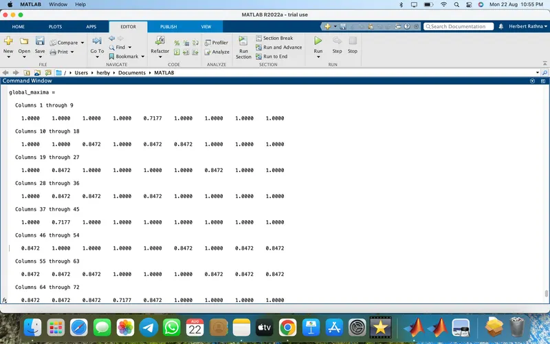
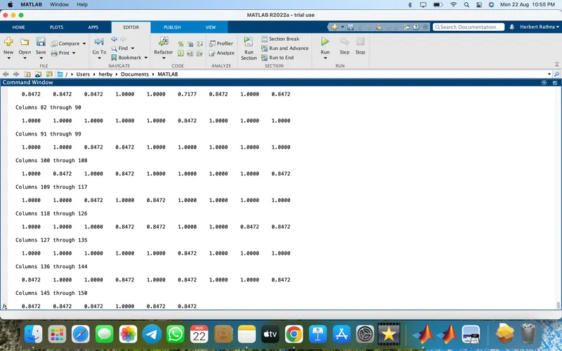
global_maxima = -fopt  

ERROR FACED:

• 'ga' function required global tool box : solved by installing add ons to the matlab

Results:

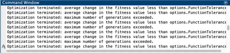
• The results show the generation of the stalagmites.

• Stalagmite Function:

• The random sampling output is shown below:

• The Bounded samples outputs are shown below:

• The bounded samples with the increased population size are shown below:

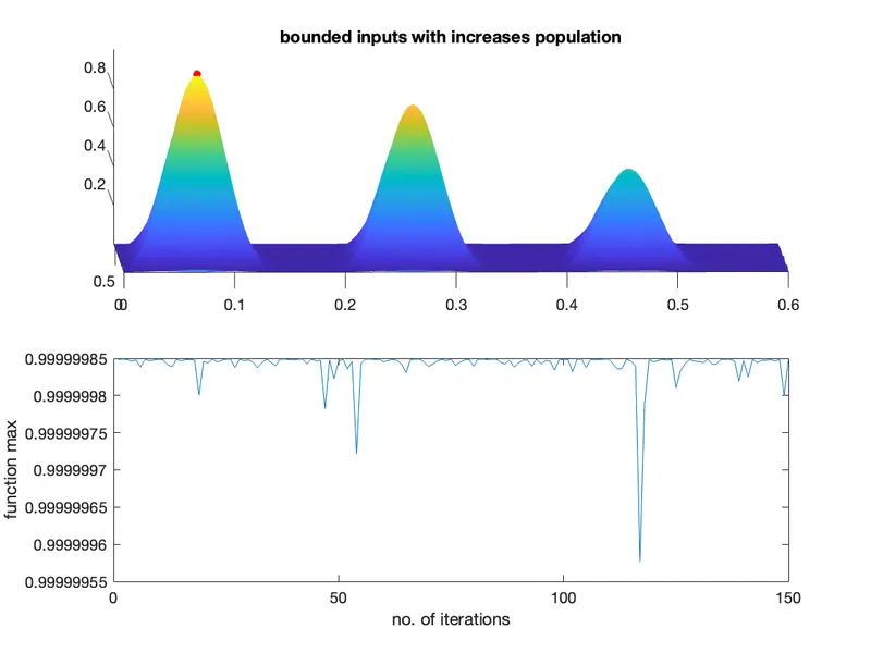
• The above- mentioned results indicate that the population size and bound samples have an optimal solutions. This is so that the code can display random samples that may begin and end at random positions.
• To overcome the issue, the bounded samples method is used giving the lower and upper limits.
• It will therefore use values that are either greater than the upper bound or less than the lower bound.The Global maximum of a function can be found by inverting the function. Find the minimum value of the inverted function, the negative of the minimum value will give the global maximum of the function.

Conclusion:

• The code to find the global maxima of the given function is written and executed successfully.
• Genetic algorithm definition,uses and its syntax is explained.
• Plotting of maximum function value verse iteration is done.

Refference:

• https://www.iitg.ac.in/rkbc/CE602/CE602/Genetic%20Algorithms.pdf
• http://www.cs.cmu.edu/~02317/slides/lec_8.pdf
• http://www.cs.cmu.edu/~02317/slides/lec_8.pdf