Week 1- Mixing Tee

REPORT Week 1 – Mixing Tee

AIM

To simulate a steady-state flow of air through mixing tee to compare the mixing effectiveness and understand the effect of length of pipe and momentum ratio of velocity for mixing of air of variant temperatures.

CASES

CASE 1

• Short mixing tee with a hot inlet velocity of 3m/s.
• Momentum ratio of 2, 4.

CASE 2

• Long mixing tee with a hot inlet velocity of 3m/s.
• Momentum ratio of 2, 4.

Momentum ratio = velocity at cold inlet / velocity at hot inlet

Value of inlet temperatures

• The hot inlet temperature is 36⁰C
• The cold inlet is at 19⁰C

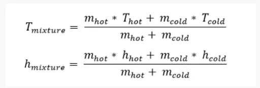
Formula

T-joint

T-Joint is a flow control device. It splits the flow with an angle between as 90 degrees. A mixing tee is a type of mixing mechanism. Mixing tee utilises a specifically engineered internal geometry to efficiently mix two fluid streams into one combined stream.

Mixing tees – in which two fluid streams with different physical, and chemical properties mix – are widely used in industries.

Hot air flowing in the main pipe is mixed with cold air flowing through a T – joint. The standard deviation of temperature is computed to quantify the degree of mixing. The velocity and temperature fields are computed. The effects of the mesh size and turbulence model on results are examined.

CASE setup

Establishing workflow

CAD cleanup/Pre-processing-SpaceClaim

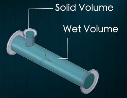
The CAD model is imported into SpaceClaim. The model is solid. To capture the fluid volume, fluid volume extraction utility in SpaceClaim by selecting the edges of 2 inlets and an outlet is done. There are two types of volume: Wet volume and solid volume. Targeted wet volume is the volume occupied by fluid.

Mesh Setup

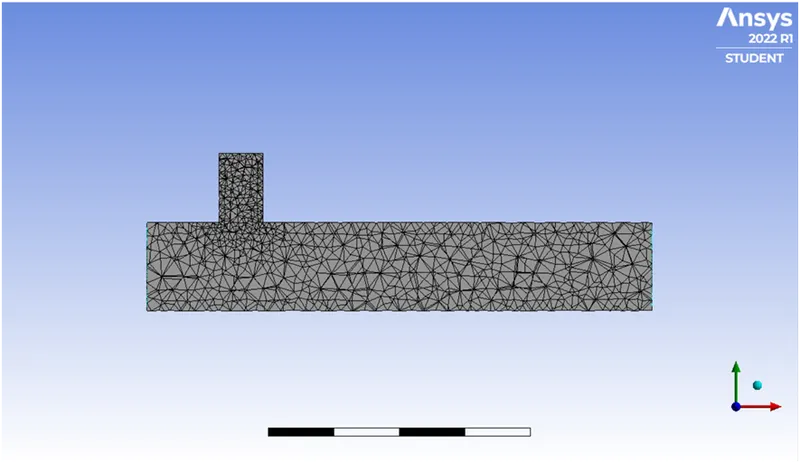
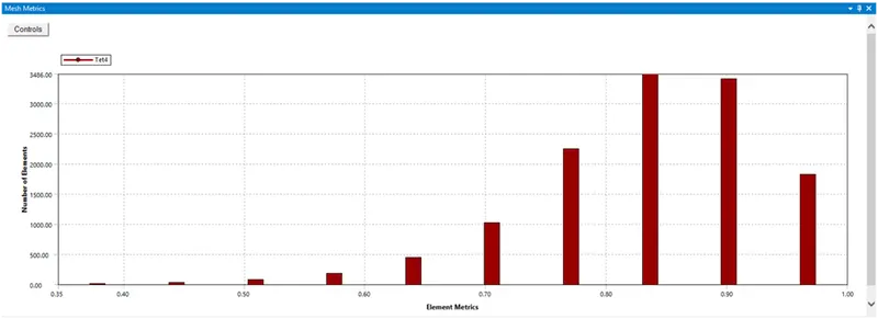
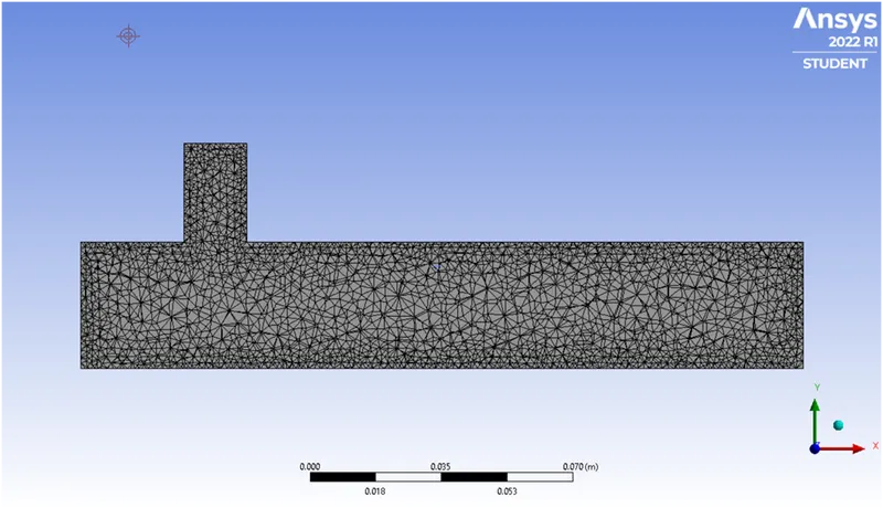
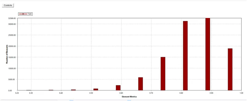
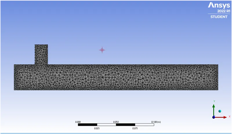
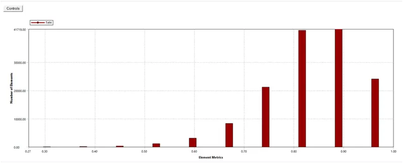
Ansys mesher is used to generate the mesh. Tetrahedral mesh is created with inflammation layers to capture the boundary layers. Although hexahedral mesh can also be used while having better quality but the tetrahedral mesh can do the job. Here, simulation quality and orthogonality and skewness are further checked.

Fluent Setup

In this setup, initial conditions, boundary conditions and numeric for the problem are set up.

• A steady-state solver is employed in a pseudo transient mode.
• Turbulence models for the cases are used, namely, the k-epsilon and the k-omega SST models.
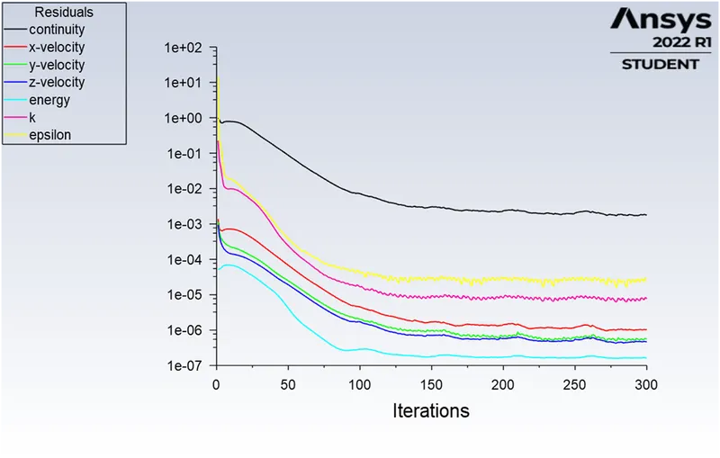
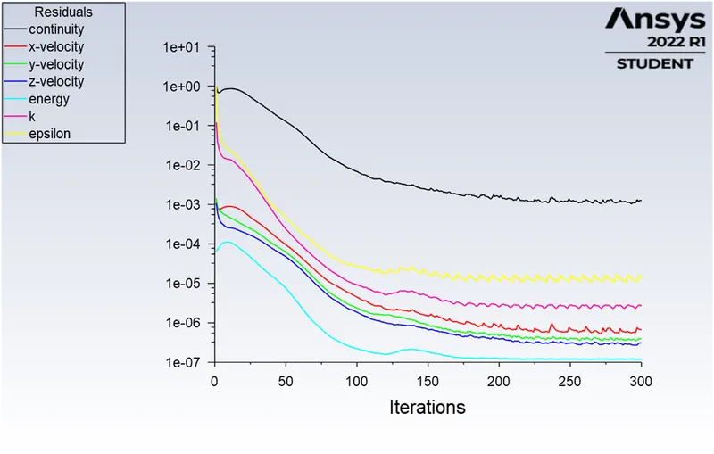
• Convergence criteria are set up.
• The number of iterations is defined here.

Post Processing

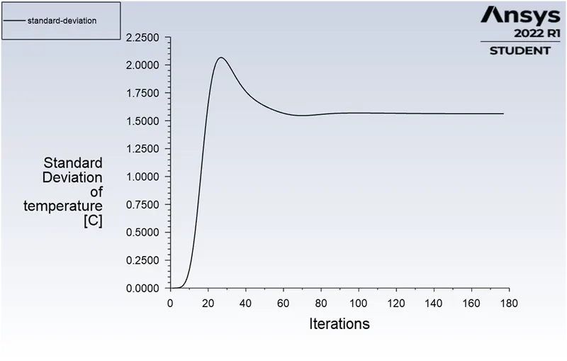
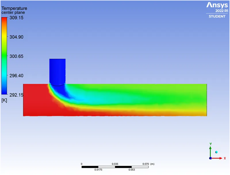
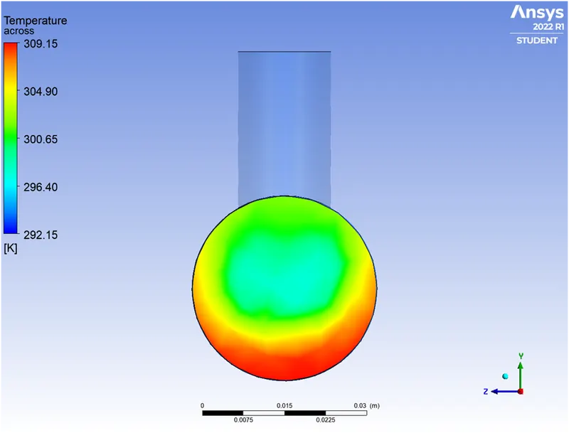
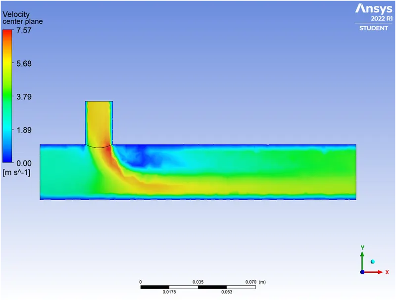
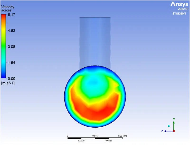
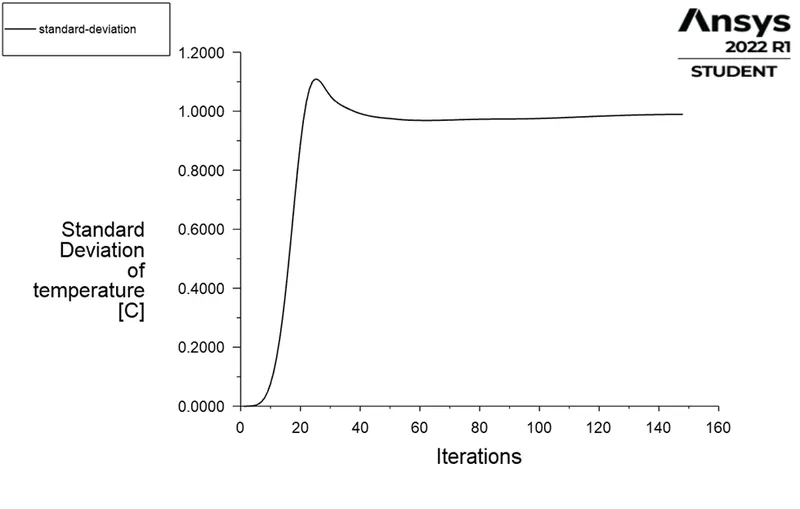
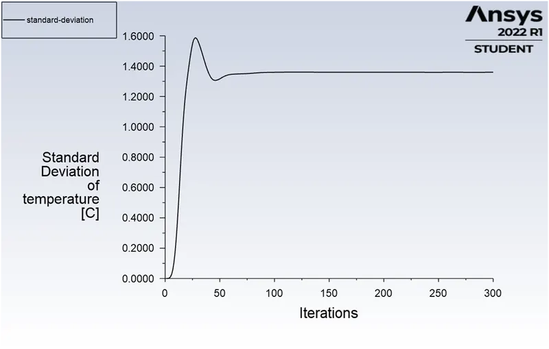
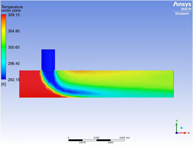
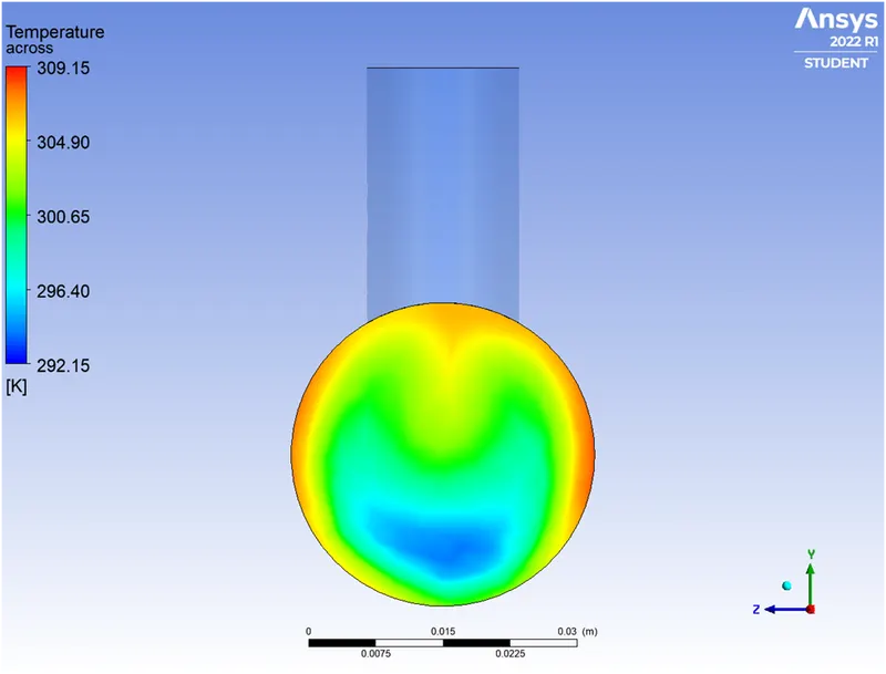
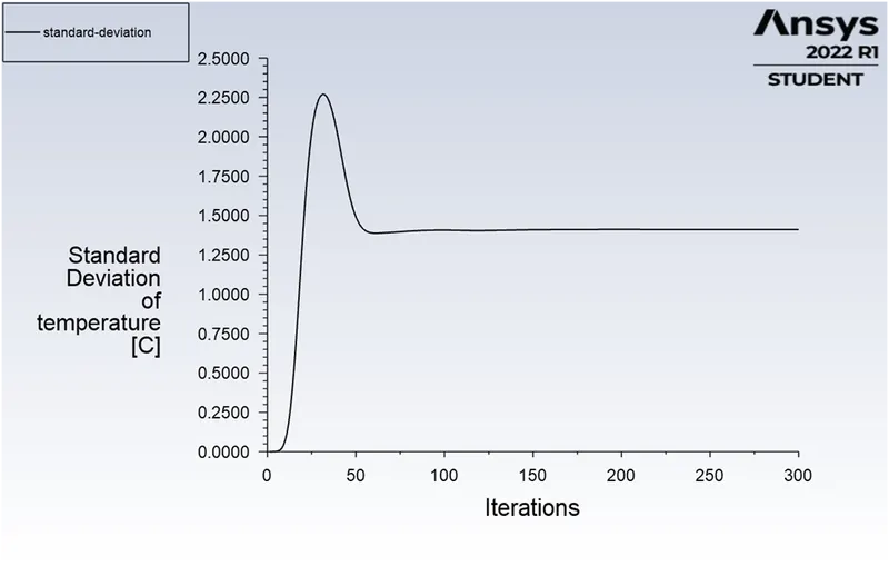
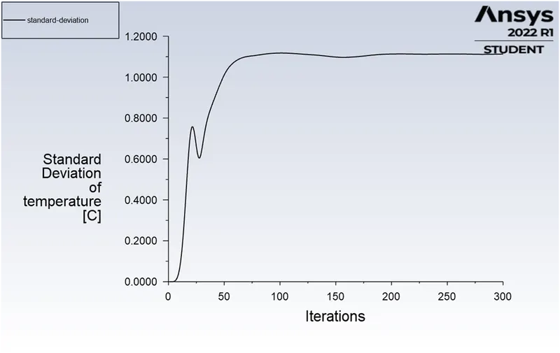
Post-processing is carried out in which different contours are set up to visualize the properties such as temperature, and velocity. For measuring the effectiveness of simulated flow through mixing tee, elementary statics is considered. The standard deviation of the temperature at the outlet is calculated to measure the effectiveness of mixing. A high standard deviation means the mixing is bad and vice versa.

SIMULATION

CASE 1 - Short Mixing Tee

Default mesh – 0.010219 m

• Hot inlet velocity of 3m/s and momentum ratio of 2

SOLVER

• Type – pressure based
• Velocity Formulation – Absolute
• Time – steady

Turbulence Model

• Model – k-epsilon (2 equation)
• K- epsilon Model – Realizable
• Near – wall Treatment – Standard Wall Functions

Material – air

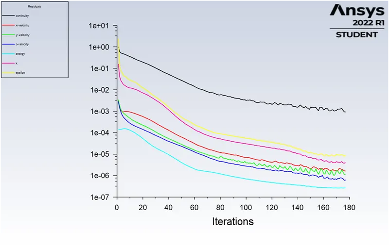
No. of iterations = 300

Solution

Line plots

Residual plot

Standard Deviation

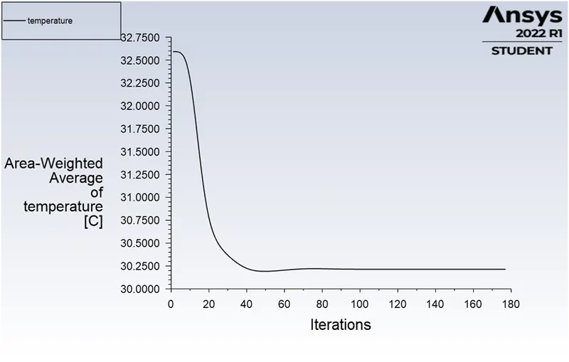
Temperature

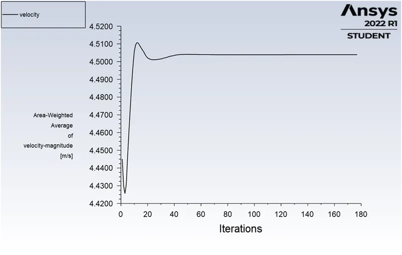
Velocity

Contour Plots

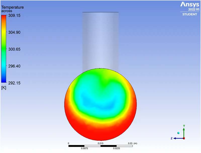
Temperature

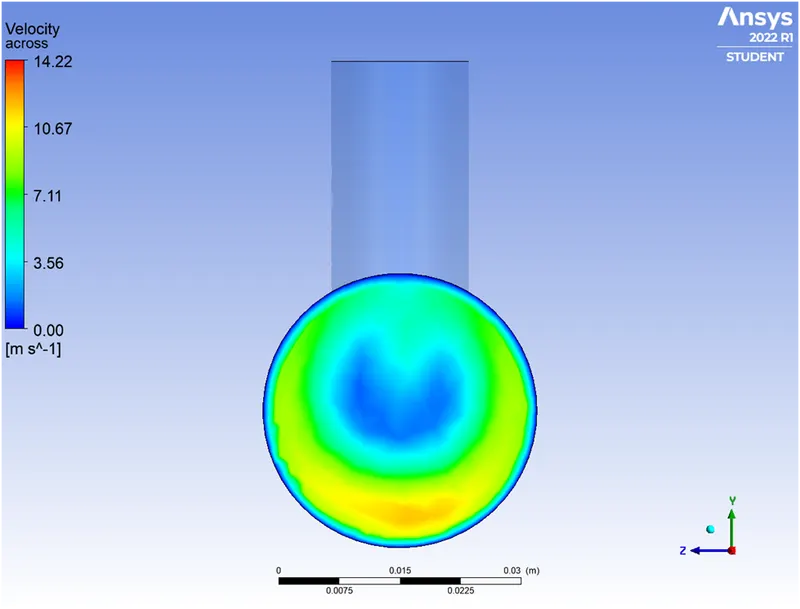
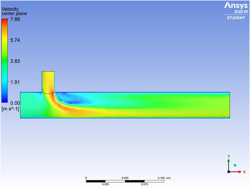
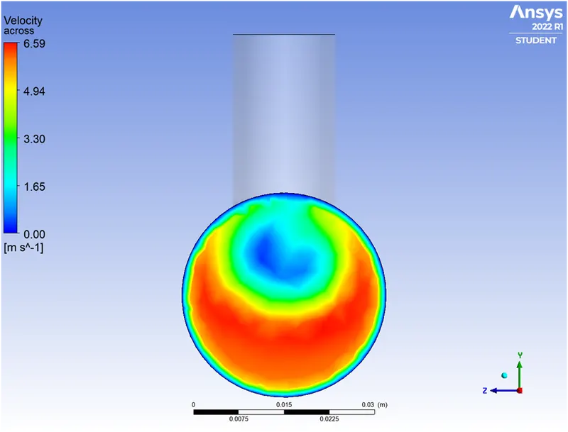
Velocity

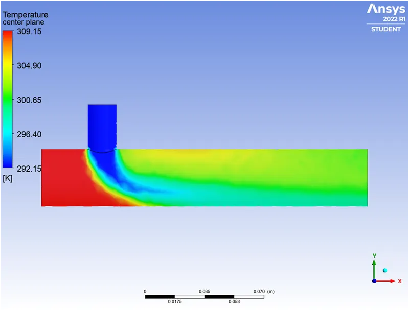
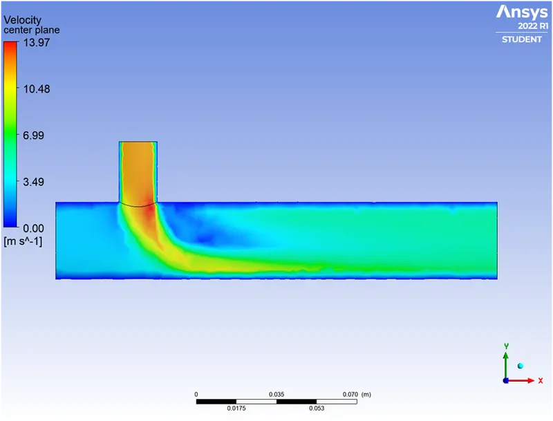
• Hot inlet velocity of 3m/s and momentum ratio of 4

SOLVER

• Type – pressure based
• Velocity Formulation – Absolute
• Time – steady

Turbulence Model

• Model – k-epsilon (2 equation)
• K- epsilon Model – Realizable
• Near – wall Treatment – Standard Wall Functions

Material – air

No. of iterations = 300

Solution

Line plots

Residual plot

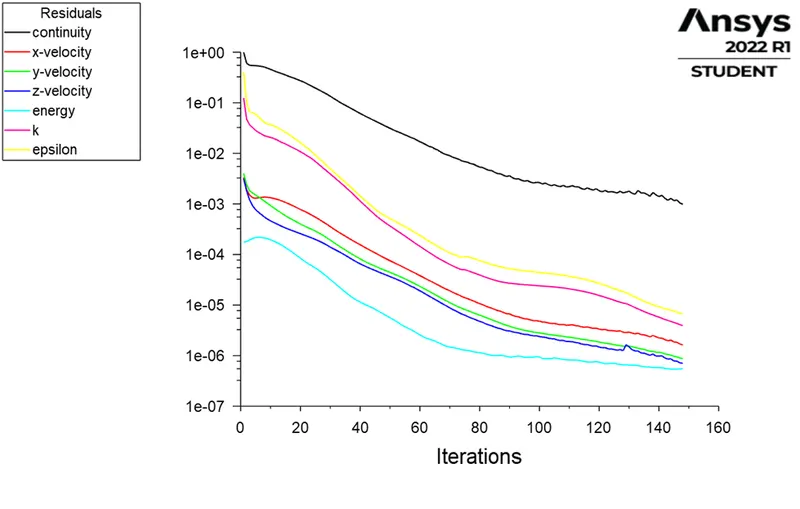
Standard Deviation

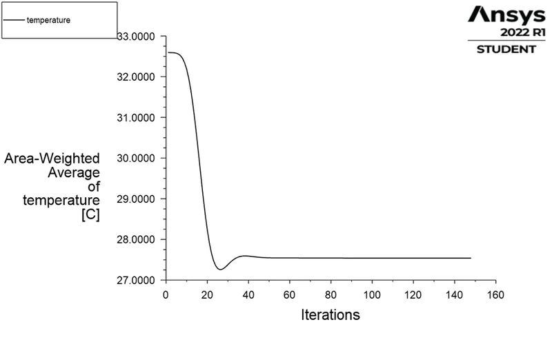
Temperature

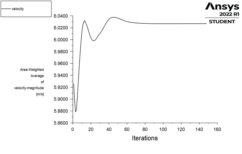
Velocity

Contour Plots

Temperature

Velocity

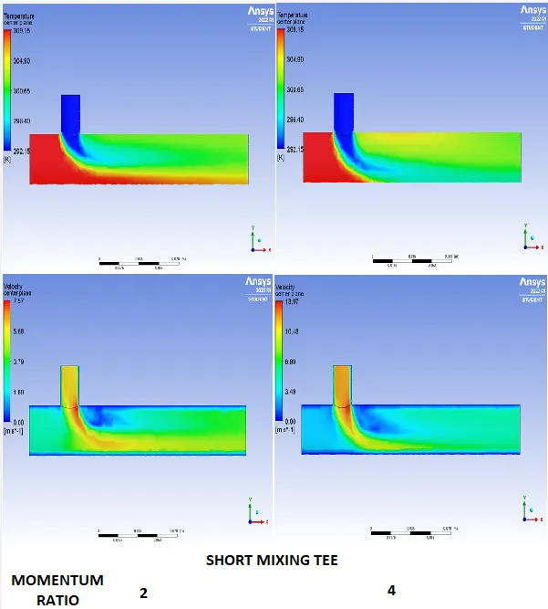
SHORT MIXING TEE

GRID INDEPENDENCE TEST

SHORT MIXING TEE

Hot inlet velocity of 3m/s and momentum ratio of 4

• Mesh Size – 0.002 m

SOLVER

• Type – pressure based
• Velocity Formulation – Absolute
• Time – steady

Turbulence Model

• Model – k-epsilon (2 equation)
• K- epsilon Model – Realizable
• Near – wall Treatment – Standard Wall Functions

Material – air

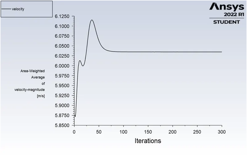
No of iterations = 300

Solution

Line plots

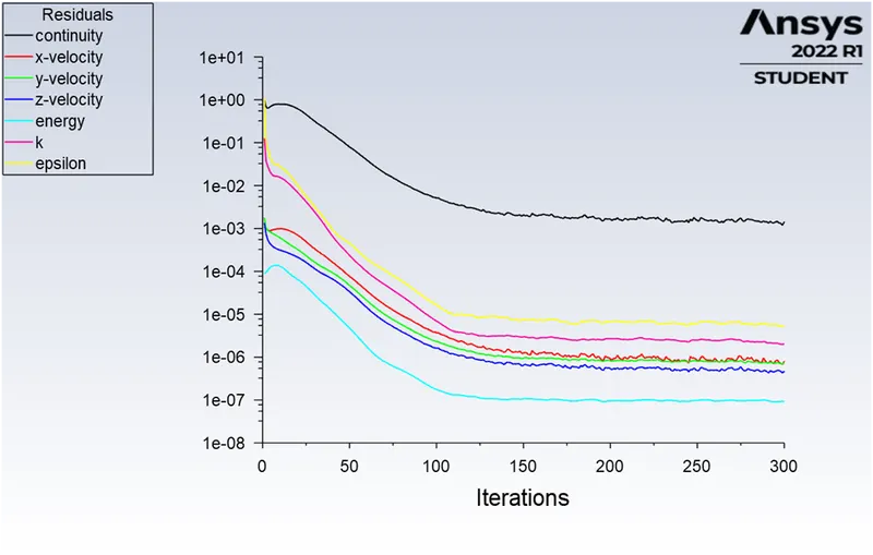
Residual plot

Standard Deviation

Temperature

Velocity

Contour Plots

Temperature

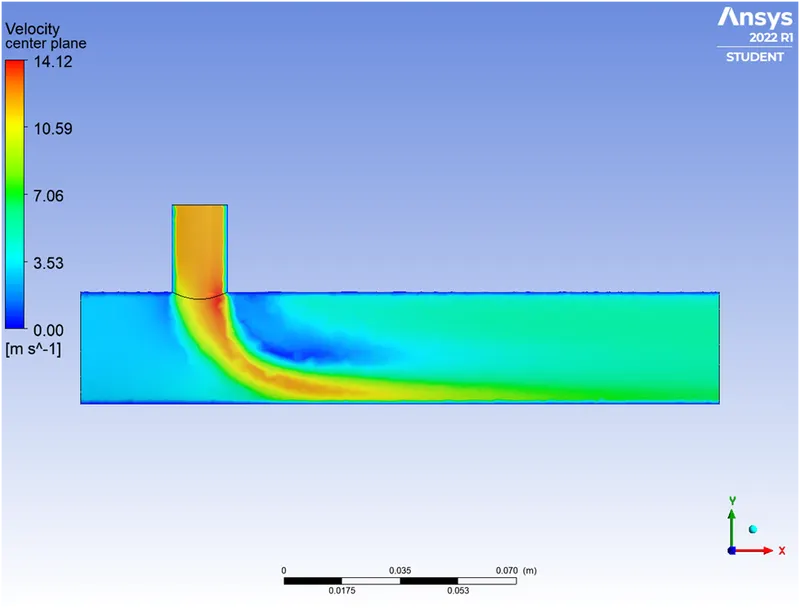
Velocity

CASE 2 - Long Mixing Tee

Default mesh – 0.002 m

• Hot inlet velocity of 3m/s and momentum ratio of 2

SOLVER

• Type – pressure based
• Velocity Formulation – Absolute
• Time – steady

Turbulence Model

• Model – k-epsilon (2 equation)
• K- epsilon Model – Realizable
• Near – wall Treatment – Standard Wall Functions

Material – air

No of iterations - 300

Solution

Line plots

Residual plot

Standard Deviation

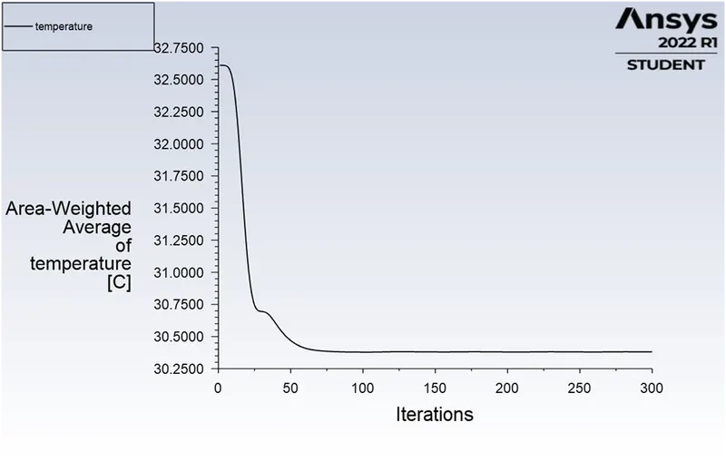
Temperature

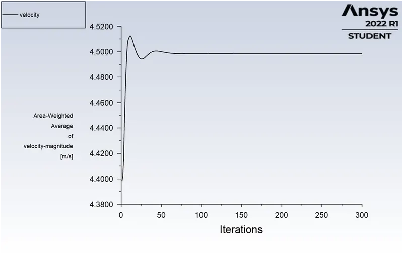
Velocity

Contour Plots

Temperature

Velocity

• Hot inlet velocity of 3m/s and momentum ratio of 4

SOLVER

• Type – pressure based
• Velocity Formulation – Absolute
• Time – steady

Turbulence Model

• Model – k-epsilon (2 equation)
• K- epsilon Model – Realizable
• Near – wall Treatment – Standard Wall Functions

Material – air

Solution

Line plots

Residual plot

Standard Deviation

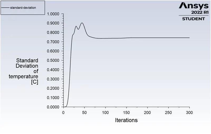
Temperature

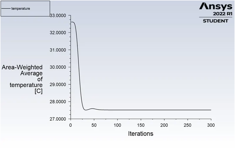
Velocity

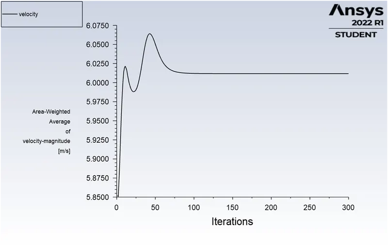
Contour Plots

Temperature

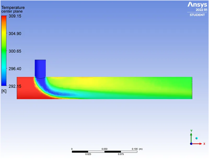
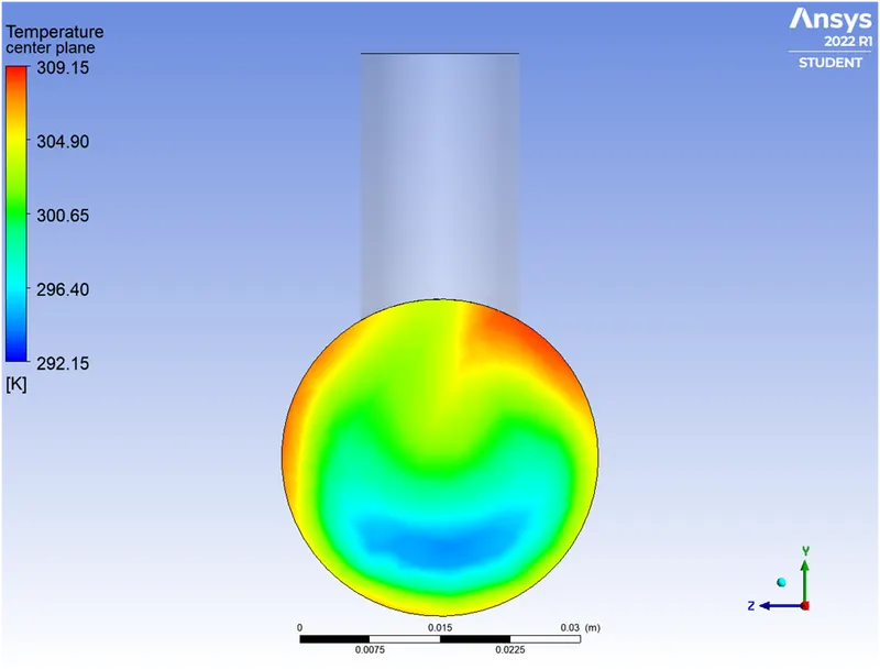
Velocity

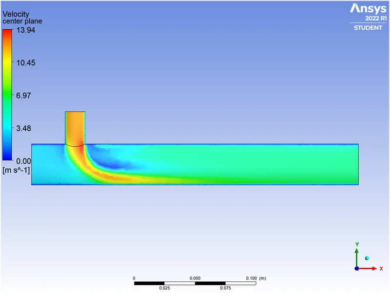
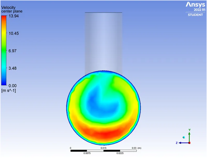
LONG MIXING TEE

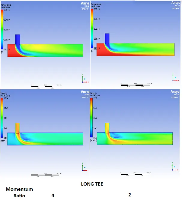
TURBULENCE MODEL

• Hot inlet velocity of 3m/s and momentum ratio of 4

SOLVER

• Type – pressure based
• Velocity Formulation – Absolute
• Time – steady

Turbulence Model

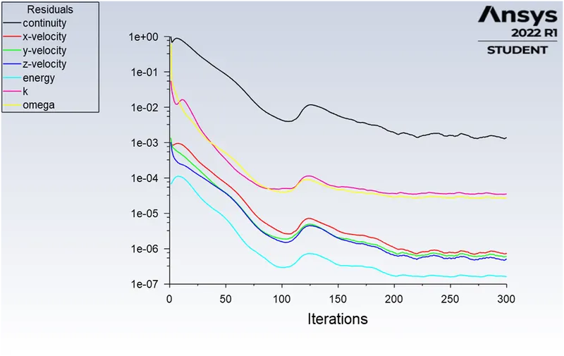
• Model – k-omega (2 equation)
• K- omega Model – SST
• K- omega Options - LowRe Corrections
• Options Production Limiter

Material – air

No of iterations - 300

Solution

Line plots

Residual plot

Standard Deviation

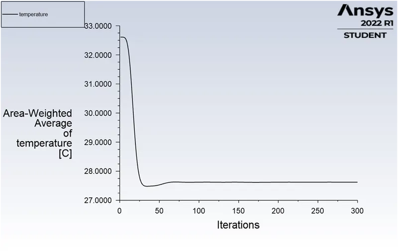
Temperature

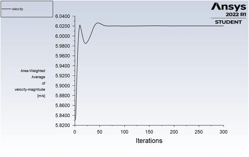
Velocity

Contour Plots

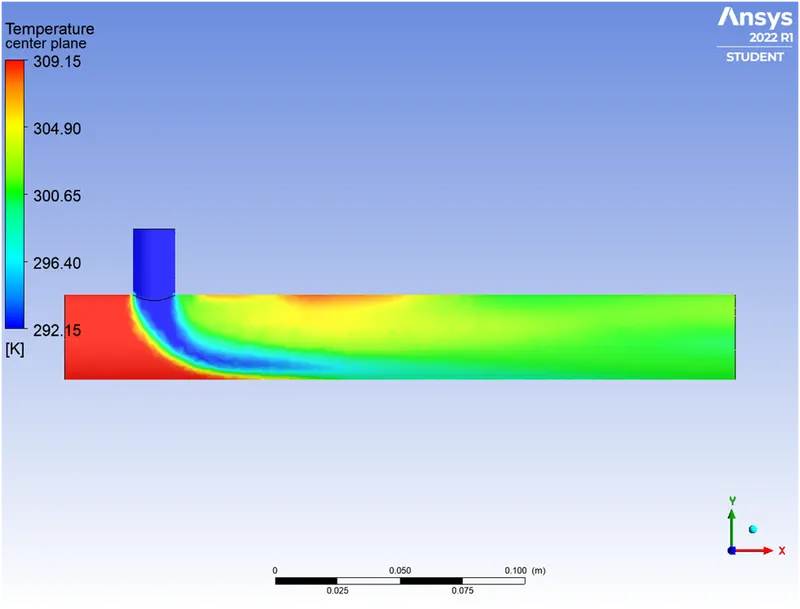
Temperature

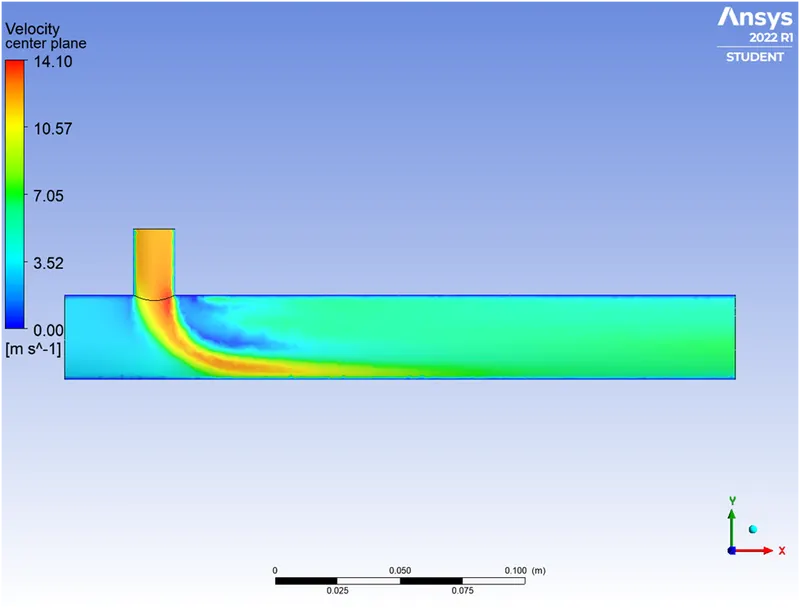
Velocity

COMPARISON

	CASE	Cell Count	Average Outlet Temperature	Number of Iterations for convergence
	SHORT TEE Momentum ratio 2	12705	30.215	180 - 200
	SHORT TEE Momentum ratio 4	12705	27.540	150
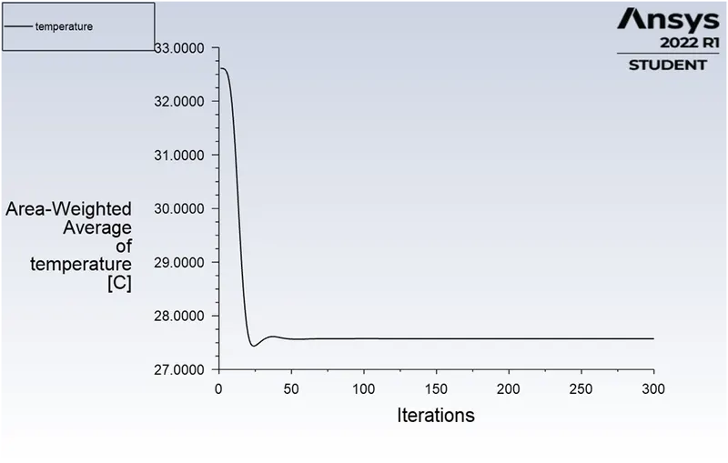
MESH INDEPENDENT TEST	Short Tee Momentum Ratio 4	106253	27.574	160 - 200
	LONG TEE Momentum ratio 2	140942	30.381	170 - 200
	LONG TEE Momentum ratio 4	140942	27.518	175
TURBULENCE MODEL	Long Tee Momentum Ratio 4	140942	27.623	250 - 275

HIGHLIGHTS

• A mesh element metric that identifies the quality of mesh was employed after mesh generating. The mesh elements with lowest quality are minimum and the quality ranges above 5 percent which is highly accepted quality.
• The boundary conditions are set as hot inlet as 36⁰C and cold inlet as 19⁰C and the cold inlet velocity is calculated by momentum ratio.
• Repot with standard deviation and area weighted average for variables like temperature, velocity were generated for each case respectively.
• For post processing plane was set up along and across the length of mixing tee and variables like temperature, velocity were noted.
• Majority of mixing (primary mixing) occurs because of higher velocity and as move along the length of the pipe there is additional mixing that occurs because of diffusion but not that dominate.
• Mesh elements were increased and the simulation was performed to check the further accuracy of the mixing.
• Two turbulence models were considered during the simulations.

CONCLUSION

MESH INDEPENDENT

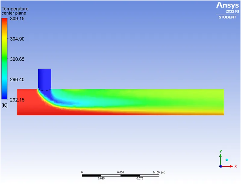
• Velocity of chilled air is very important. As it can seen that the outlet temperature drops significantly due to high velocity of the cold air from the inlet-y. By increasing the speed of chilled air we can reduce the outlet temperature easily as we get better turbulent mixing.
• The contour plot of temperature shows that some of the high temperature flow slips through without mixing properly with the chilled flow.
• So, large momentum ratio of the flow provides better mixing.
• The longer configuration is not effective significantly on the outlet conditions as the temperature of mixed fluid becomes uniformly distributed due to turbulent nature of the flow.
• The standard deviation of temperature in case of longer tee is low as compared to short tee for both momentum ratios.
• Mesh independent test allows mesh refinement without affecting results as can be seen from the result plots.
• K-epsilon can be chosen for better results as the solution is converged after lesser iterations as compared with k-omega model.
• K-epsilon turbulence model is the most common model used in CFD to simulate mean flow characteristics for turbulent flow conditions. It is a two equation model that gives a general description of turbulence by means of two transport equations. K-epsilon model is ideal for predicting flow behavior in regions away from the wall.
• The SST k-omega turbulence model is a two-equation eddy-viscosity model that is used for many aerodynamic applications. The k-omega model is well suited for simulating flow in the viscous sub-layer. The SST models exhibit less sensitivity to free stream conditions ( flow outside the boundary layer) than many other turbulence models.