Week 9 - FVM Literature Review

REPORT  FVM Literature Review

OBJECTIVE

• What is the Finite Volume Method (FVM)?
• Major differences between FDM & FVM.
• Describe the need for the interpolation schemes and flux limiters in FVM.
• Explain with an example of a 1D linear heat conduction equation.

DESCRIPTION

FINITE VOLUME METHOD

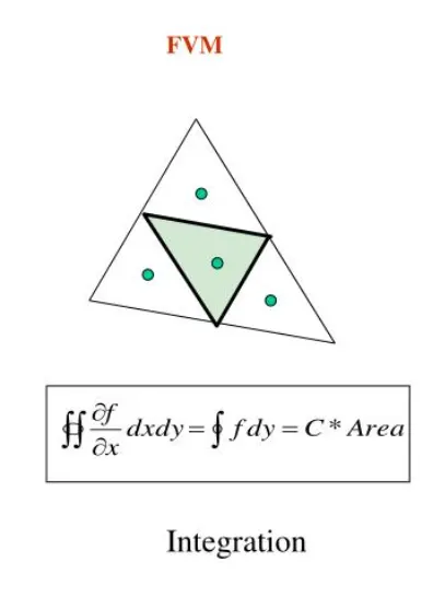
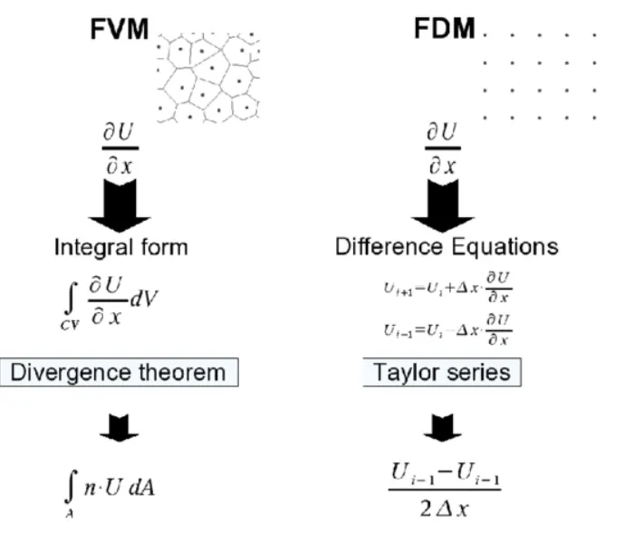
The finite volume method is a widely used numerical technique. Finite volume refers to the small volume surrounding each node point on a mesh. FVM transforms the set of partial differential equations into a system of linear algebraic equations. In the finite volume method, volume integrals are introduced in a partial differential equation, they contain a divergence term that is converted to surface integrals, using the divergence theorem. These terms are then evaluated as fluxes at the surfaces of each finite volume. Because the flux entering a given volume is identical to that leaving the adjacent volume, these methods are conservative.

FVM is similar to FDM but the method (FVM) integrates the differential equation over a control volume and discretizes the domain. Since we have integrated the differential equation discretization is mathematically a valid one. Although the discrete approximation procedure used in the FVM is distinctive, it also utilizes the basic steps. In both cases, the values of field variables at non-storage locations (e.g. vertices) are obtained using interpolation.

Although the discrete approximation procedure used in the FVM is distinctive, it is also utilized in basic steps. Firstly, it transforms and integrated the PDEs into balance equations over an element. The process incorporates the changing of the surface and volume integrals into discrete algebraic relations over elements as well as their surfaces in an integration quadrature of a specified order of accuracy. This will result in a set of semi-discrete equations. Secondly, in this next step, the interpolation profiles are chosen to estimate the variation of the variables within the element and relate the surface values of the variables to their cell values and thus transform the algebraic relations into algebraic equations. In regards to the two steps in the FVM process, your approximation selection affects the overall accuracy of the subsequent numeric.

The gauss or divergence theorem simply states that the outward flux of a vector field through a closed surface is equal to the volume integral of the divergence over the region inside the surface. This theorem is fundamental in the FVM, it is used to convert the volume integrals appearing in the governing equation into surface integrals. The face values appearing in the convective and diffusive fluxes have to be computed by some form of interpolation from the centroid values of the control volume at both sides of the face.

Advantages of FVM

The advantage of the finite volume method is that it is easily formulated to allow for unstructured meshes. The method is used in many CFD packages. The FVM's most significant advantage is that it only needs to do flux evaluation for the cell boundaries. Also, this is true for nonlinear issues as well, which, in turn, makes it an excellent choice for the handling of (nonlinear) conservation laws.

FDM

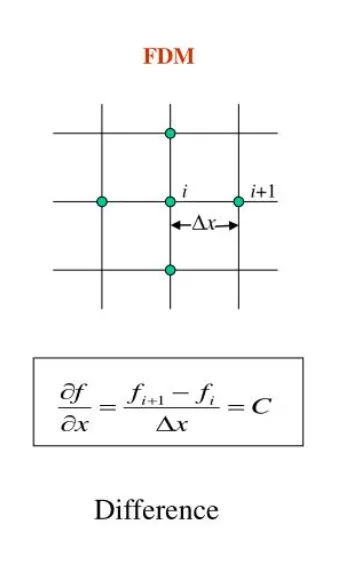
A finite difference method (FDM) discretization is based upon the differential form of the PDE to be solved. Each derivative is replaced with an approximate difference formula (that can generally be derived from a Taylor series expansion). The computational domain is usually divided into hexahedral cells (the grid), and the solution will be obtained at each nodal point. The FDM is easiest to understand when the physical grid is cartesian, but through the use of curvilinear transforms the method can be extended to domains that are not easily represented by brick-shaped elements. The discretization results in a system of equations of the variable at nodal points, and once a solution is found, then we have a discrete representation of the solution.

FDM vs FVM

Finite Volume Method (FVM)	Finite Difference Method (FDM)
FVM is straightforward to implement on a non-uniform/ unstructured grid.	FDM requires a specific type of grid.
The dependant variable values are stored at the nodes only.	The dependant values are stored at the element nodes.
FVM discretizes the integral form of the balance equations. This gives special care (mass conservative or momentum conservative) in FVM is more natural and guaranteed compared to FDM.	FDM solves using the differential form.
It can be shown that is equivalent to using a weak formulation, the only one that can be adopted for non-regular solutions.	FDM cannot be used because the derivatives cannot be defined across a discontinuity.
In the FV approach, conservation of mass, this momentum, and energy are ensured at each cell/ finite volume level.	FDM mostly requires regular domains with uniform meshing.
Handling shocks (discontinues in solution or space or material) in the integral form of balance equations is easier.	Discontinuities in solution or space or material (like shocks) are harder to handle in differential forms.
The basic advantage of FVM over FDM is it requires the use of structured grids, and the effort to convert the given mesh in the structured numerical grid internally is completely avoided.	As with FDM, the resulting approximate solution is discrete, but the variables are typically placed at cell centres rather than at nodal points.

Need for Interpolation Schemes and Flux Limiters in FVM

• Interpolation Schemes

Interpolation is a type of estimation, a method of constructing (finding) new data points based on the range of a discrete set of known data points. Interpolation schemes are used to transform cell-centre quantities to face centres. The operation is used in many finite volume calculations, e.g. for the calculation of gradient, divergence, and Laplacian terms.

Interpolation schemes approximate the property values located at the boundaries of the control volumes which are necessary when FVM is applied. The correspondent properties located at the centre of the adjacent control volumes are calculated using interpolation nodes. The approximations of surface and volume integrals require values of the variable at locations other than the computational nodes of the CV. Values at these locations are obtained using interpolation formulae.

• Flux Limiters

Flux limiters are used in high-resolution schemes – numerical schemes used to solve problems in engineering, particularly fluid dynamics, described by partial differential equations. They are used in high-resolution schemes, such as the MUSCL scheme, to avoid the spurious oscillations (wiggles) that would otherwise occur with high order spatial discretization schemes due to shocks, discontinuities or sharp changes in the solution domain. The use of flux limiters, together with an appropriate high-resolution scheme, makes the solution's total variation diminishing (TVD). Note that flux limiters are also referred to as slope limiters because they both have the same mathematical form, and both have the effect of limiting the solution gradient near shocks or discontinuities. In general, the term flux limiter is used when the limiter acts on system fluxes, and slope limiter is used when the limiter acts on system states (like pressure, velocity etc.).

The idea is to tune the numerical flux of high order and low order schemes using the flux limiter function in such a way that the resulting scheme gives a high order accuracy in the smooth region of  flow and sticks with the first-order accuracy in the vicinity of socks/ discontinuities as follows:

Define the numerical flux function of a high-resolution conservative scheme as

Where L and H are the numerical flux of conservative low order and high order schemes respectively. And `phi` is a function of the smoothness parameter `theta` usually defines as

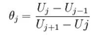
Limiter function `phi(theta)` in such a way that it satisfies at least the following properties:

• Remains positive for all `theta`
• Satisfies `phi`(1) = 1
• Passes through a particular region known as the TVD region associated with the underlying scheme to guarantee the stability of the scheme.