Week 3.5 - Deriving 4th order approximation of a 2nd order derivative using Taylor Table method

REPORT – Deriving 4^th order approximation of a 2^nd order derivative using the Taylor method

AIM

Derive the following 4^th order approximations of the second-order derivative.

• Central difference
• Skewed right-sided difference
• Skewed left-sided difference

OBJECTIVE

After deriving these schemes,

• Prove that the skewed schemes are fourth-order accurate.
• Write a program in Matlab to evaluate the second-order derivative of the analytical function exp(x) * cos(x) and compare it with the 3 numerical approximations that you have derived.
• Provide a plot that compares the absolute error between the mentioned schemes.
• Describe why a skewed scheme is useful. What can a skewed scheme do that a CD scheme cannot.

HINT GIVEN

• The order of accuracy P = Number of nodes in the stencil N – order of derivative Q + 1 for symmetric/central schemes.
• The order of accuracy P = Number of nodes in the stencil N – order of derivative Q for one-sided/ skewed schemes.
• Solve the system of equations using the matrix inversion method in Matlab to obtain the Taylor table coefficients and use them directly in the numerical approximation statements to avoid input errors.

EXPLANATION

CFD is the analysis of physical systems like fluid flow and heat transfer by performing computer-based simulations. We take up a system, find the underlying governing differential equations, and determine suitable numerical methods to approximate them. A numerical approximation is necessary because a problem in differential equations can rarely be solved analytically. Taylor table method is another numerical approximation method to compute the derivatives of the function. In the Taylor table method, we find numerical schemes to meet the target accuracy.

Nomenclature;

• P - Order of approximation
• Q - Order of derivative
• dx (also represented as `/_x`) - represents the difference of two consecutive nodes;

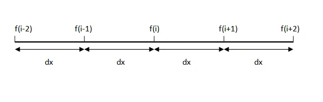
Here,

Function is `f(x) = e^x * cos(x)`

To calculate 4^th order approximation of 2^nd order derivative of function f(x);

Here, P = 4 and Q = 2

Taylor series general equation:

`f(x + dx) = f(x) + (del f)/(del x) *dx + (del^2f(x))/(delx^2) *(dx)^2/(2!) + ... + (del^nf(x))/(delx^n) * (dx)^n/(n!) + …`

Therefore,

• Central Difference

For central schemes; no of nodes = P + Q -1 = 4 + 2 – 1 = 5

Nodes considered: [i -2, i -1, i, i +1, i+2]

Hypothesis equation

`(/_x)^2 * (d^2 f)/(dx^2) = a*f(i - 2) + b*f(i - 1) + c*f(i) + d*f(i + 1) + e*f(i + 2)`

According to the Taylor series;

• `a*f(i - 2) = a*(f(i) - (2/_x)/(1!) * f'(i) + (2/_x)^2/(2!) * f''(i) - (2/_x)^3/ (3!) * f'''(i) + (2/_x) ^4/(4!) * f''''(i))`
• `b*f (i - 1) =b*(f(i) - (/_x)/(1!) * f'(i) + (/_x)^2/(2!) * f''(i) - (/_x)^3/(3!) * f'''(i) + (/_x)^4/(4!) * f''''(i))`
• `c*f(i)`
• `d*f(i + 1) = d*(f(i) + (/_x)/(1!) * f'(i) + (/_x)^2/(2!) * f''(i) + (/_x)^3/(3!) * f'''(i) + (/_x)^4/(4!)* f''''(i))`
• `e*f(i + 2) = e*(f(i) + (2/_x)/(1!) * f'(i) + (2/_x)^2/(2!) * f''(i) + (2/_x)^3/(3!) * f'''(i) + (2/_x)^4/(4!) * f''''(i))`

TAYLOR TABLE

Table Series Terms	`f(i)`	`(/_x)*f'(i)`	`(/_x)^2*f''(i)`	`(/_x)^3*f'''(i)`	`(/_x)^4*f''''(i)`
Stencil
`a*f(i - 2)`	a	-2a	4a/2	-8a/6	16a/24
`b*f(i - 1)`	b	-b	b/2	-b/6	b/24
`c*f(i)`	c	0	0	0	0
d*f(i + 1)	d	d	d/2	d/6	d/24
`e*f(i + 2)`	e	2e	4e/2	8e/6	16e/24

Summing the respective columns provide us;

• a + b + c + d + e + g = 0
• -2a – b + d + 2e = 0
• 4a/2 + b/2 + d/2 + 4e/2 = 1
• -8a/6 – b/6 + d/6 + 8e/6 = 0
• 16a/24 + b/24 + d/24 + 16e/24 = 0

Code for solving the above mentioned 6x6 linear equations;

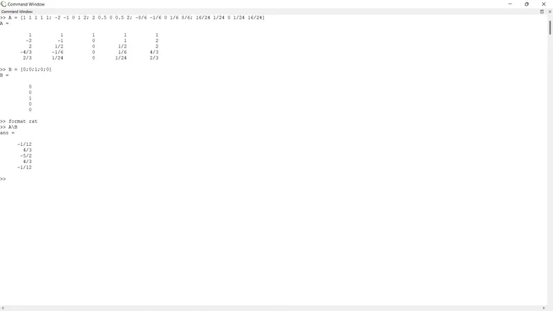
Thus, values are as follows:

a = -0.083333 = -1/12

b = 1.333333 = 4/3

c = -2.500000 = -5/2

d = 1.333333 = 4/3

e = -0.083333 = -1/12

Therefore, equation becomes

`(/_x)^2 * (d^2 f)/(dx^2) = a*f(i - 2) + b*f(i - 1) + c*f(i) + d*f(i + 1) + e*f(i + 2)`

`(/_x)^2 * (d^2 f)/(dx^2) = (-0.083333)*f(i - 2) + (1.333333)*f(i - 1) + (-2.500000)*f(i) + (1.333333)*f(i + 1) + (-0.083333)*f(i + 2)`

• Skewed right- sided difference

For skewed schemes; no of nodes = P + Q = 4 + 2 = 6

Nodes consider: [i, i + 1, i + 2, i +3, i + 4, i + 5]

Hypothesis equation

`(/_x)^2 * (d^2 f)/(dx^2) = a*f(i) + b*f(i + 1) + c*f(i + 2) + d*f(i + 3) + e*f(i + 4) + g*f(i + 5)`

According to the Taylor series;

• `a*f(i)`
• `b*f (i + 1) =b*(f(i) + (/_x)/(1!) * f’(i) + (/_x)^2/(2!) * f''(i) + (/_x)^3/(3!) * f'''(i) + (/_x)^4/(4!) * f''''(i) + (/_x)^5/(5!) * f'''''(i))`
• `c*f(i + 2) = c*(f(i) + (2/_x)/(1!) * f'(i) + (2/_x)^2/(2!) * f''(i) + (2/_x)^3/(3!) * f'''(i) + (2/_x)^4/(4!) * f''''(i) + (2/_x)^5/(5!) * f'''''(i))`
• `d*f(i + 3) = d*(f(i) + (3/_x)/(1!) * f'(i) + (3/_x)^2/(2!) * f''(i) + (3/_x)^3/(3!) * f'''(i) + (3/_x)^4/(4!) * f''''(i) + (3/_x)^5/(5!) * f'''''(i))`
• `e*f(i + 4) = e*(f(i) + (4/_x)/(1!) * f'(i) + (4/_x)^2/(2!) * f''(i) + (4/_x)^3/(3!) * f'''(i) + (4/_x)^4/(4!) * f''''(i) + (4/_x)^5/(5!) * f'''''(i))`
• `g*f(i + 5) = g*(f(i) + (5/_x)/(1!) * f'(i) + (5/_x)^2/(2!) * f''(i) + (5/_x)^3/(3!) * f'''(i) + (5/_x)^4/(4!) * f''''(i) + (5/_x)^5/(5!) * f'''''(i))`

TAYLOR TABLE

Table Series Terms	`f(i)`	`(/_x)*f'(i)`	`(/_x)^2*f''(i)`	`(/_x)^3*f'''(i)`	`(/_x)^4*f''''(i)`	`(/_x)^5*f'''''(i)`
Stencil
`a*f(i)`	a	0	0	0	0	0
`b*f(i + 1)`	b	b	b/2	b/6	b/24	b/120
`c*f(i + 2)`	c	2c	4c/2	8c/6	16c/24	32c/120
`d*f(i + 3)`	d	3d	9d/2	27d/6	81d/24	243d/120
`e*f(i + 4)`	e	4e	16e/2	64e/6	256e/24	1024e/120
`g*f(i + 5)`	g	5g	25g/2	125g/6	625g/24	3125g/120

Summing the respective columns provide us;

• a + b + c + d + e + g = 0
• b + 2c + 3d + 4e + 5g = 0
• b/2 + 4c/2 + 9d/2 + 16e/2 + 25g/2 = 1
• b/6 + 8c/6 + 27d/6 + 64e/6 + 125g/6 = 0
• b/24 + 16c/24 + 81d/24 + 256e/24 + 625g/24 = 0
• b/120 + 32c/120 + 243d/120 + 1024e/120 + 3125g/120 = 0

Code for solving the above mentioned 6x6 linear equations;

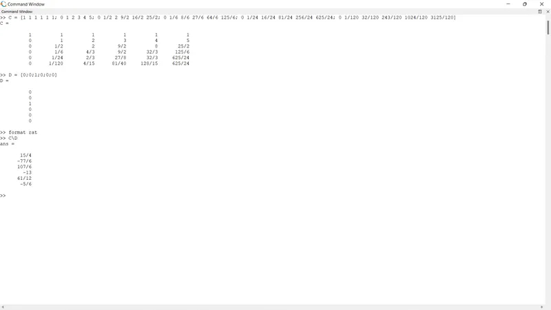
Thus, values are as follows:

a = 3.7500 = 15/4

b = -12.8333 = -77/6

c = 17.8333 = 107/6

d = -13.0000 = -13

e = 5.0833 = 61/12

f = -0.8333 = -5/6

Therefore, equation becomes

`(/_x)^2 * (d^2 f)/(dx^2) = a*f(i) + b*f(i + 1) + c*f(i + 2) + d*f(i + 3) + e*f(i + 4) + g*f(i + 5)`

`(/_x)^2 * (d^2 f)/(dx^2) = (3.7500)*f(i) + (-12.8333)*f(i + 1) + (17.8333)*f(i + 2) + (-13.0000)*f(i + 3) + (5.0833)*f(i + 4) + (-0.8333)*f(i + 5)`

• Skewed left- sided difference

For skewed schemes; no of nodes = P + Q = 4 + 2 = 6

Nodes consider: [i -5 , i - 4, i - 3, i - 2, i - 1, i]

Hypothesis equation

`(/_x)^2 * (d^2 f)/(dx^2) = a*f(i) + b*f(i - 1) + c*f(i - 2) + d*f(i - 3) + e*f(i - 4) + g*f(i - 5)`

According to the taylor series;

• `a*f(i)`
• `b*f (i - 1) = b*(f(i) - (/_x)/(1!) * f'(i) + (/_x)^2/(2!) * f''(i) - (/_x)^3/(3!) * f'''(i) + (/_x)^4/(4!) * f''''(i) - (/_x)^5/(5!) * f'''''(i))`
• `c*f(i - 2) = c*(f(i) - (2/_x)/(1!) * f'(i) + (2/_x)^2/(2!) * f''(i) - (2/_x)^3/(3!) * f'''(i) + (2/_x)^4/(4!) * f''''(i) - (2/_x)^5/(5!) * f'''''(i))`
• `d*f(i - 3) = d*(f(i) - (3/_x)/(1!) * f'(i) + (3/_x)^2/(2!) * f''(i) - (3/_x)^3/(3!) * f'''(i) + (3/_x)^4/(4!) * f'''''(i) - (3/_x)^5/(5!) * f'''''(i))`
• `e*f(i - 4) = e*(f(i) - (4/_x)/(1!) * f'(i) + (4/_x)^2/(2!) * f’’(i) - (4/_x)^3/(3!) * f'''(i) + (4/_x)^4/(4!) * f''''(i) - (4/_x)^5/(5!) * f'''''(i))`
• `g*f(i - 5) = g*(f(i) - (5/_x)/(1!) * f'(i) + (5/_x)^2/(2!) * f''(i) - (5/_x)^3/(3!) * f'''(i) + (5/_x)^4/(4!) * f''''(i) - (5/_x)^5/(5!) * f'''''(i))`

TAYLOR TABLE

Table Series Terms	`f(i)`	`(/_x)*f'(i)`	`(/_x)^2*f''(i)`	`(/_x)^3*f'''(i)`	`(/_x)^4*f''''(i)`	`(/_x)^5*f'''''(i)`
Stencil
`a*f(i)`	a	0	0	0	0	0
`b*f(i - 1)`	b	-b	b/2	-b/6	b/24	-b/120
`c*f(i - 2)`	c	-2c	4c/2	-8c/6	16c/24	-32c/120
`d*f(i - 3)`	d	-3d	9d/2	-27d/6	81d/24	-243d/120
`e*f(i - 4)`	e	-4e	16e/2	-64e/6	256e/24	-1024e/120
`g*f(i - 5)`	g	-5g	25g/2	-125g/6	625g/24	-3125g/120

Summing the respective columns provide us;

• a + b + c + d + e + g = 0
• -b - 2c - 3d - 4e - 5g = 0
• b/2 + 4c/2 + 9d/2 + 16e/2 + 25g/2 = 1
• -b/6 - 8c/6 - 27d/6 - 64e/6 - 125g/6 = 0
• b/24 + 16c/24 + 81d/24 + 256e/24 + 625g/24 = 0
• -b/120 - 32c/120 - 243d/120 - 1024e/120 - 3125g/120 = 0

Code for solving the above mentioned 6x6 linear equations;

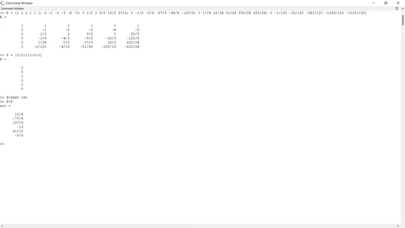
Thus, values are as follows:

a = 3.7500 = 15/4

b = -12.8333 = -77/6

c = 17.8333 = 107/6

d = -13.0000 = -13

e = 5.0833 = 61/12

f = -0.8333 = -5/6

Therefore, equation becomes

`(/_x)^2 * (d^2 f)/(dx^2) = a*f(i) + b*f(i - 1) + c*f(i - 2) + d*f(i - 3) + e*f(i - 4) + g*f(i - 5)`

`(/_x)^2 * (d^2 f)/(dx^2) = (3.7500)*f(i) + (-12.8333)*f(i - 1) + (17.8333)*f(i - 2) + (-13.0000)*f(i - 3) + (5.0833)*f(i - 4) + (-0.8333)*f(i - 5)`

CODE

TO EVALUATE THE 2nd ORDER DERIVATIVE OF FUNCTION AND COMPARE IT WITH THE CENTRAL, SKEWED RIGHT SIDED AND SKEWED LEFT SIDED NUMERICAL APPROXIMATIONS

clear all 
close all
clc

% value of x
x = pi/3;
% range of dx
dx = linspace(pi/40,pi/4000,80);

% function f(x) = exp(x)*cos(x)
% actual derivative of function = exp(x)*(cos(x) - sin(x))
% second order derivative of function = -2*exp(x)*sin(x)
analytical_derivative = -2*exp(x)*sin(x);

for k = 1:length(dx)
  
  % Taylor series terms
  A(k) = exp(x - (5*dx(k)))*cos(x - (5*dx(k)));
  B(k) = exp(x - (4*dx(k)))*cos(x - (4*dx(k)));
  C(k) = exp(x - (3*dx(k)))*cos(x - (3*dx(k)));
  D(k) = exp(x - (2*dx(k)))*cos(x - (2*dx(k)));
  E(k) = exp(x - (1*dx(k)))*cos(x - (1*dx(k)));
  F(k) = exp(x) * cos(x);
  G(k) = exp(x + (1*dx(k)))*cos(x + (1*dx(k)));
  H(k) = exp(x + (2*dx(k)))*cos(x + (2*dx(k)));
  I(k) = exp(x + (3*dx(k)))*cos(x + (3*dx(k)));
  J(k) = exp(x + (4*dx(k)))*cos(x + (4*dx(k)));
  K(k) = exp(x + (5*dx(k)))*cos(x + (5*dx(k)));
  
  % Central differencing
  central_differencing(k) = ((-1/12)*D(k) + (4/3)*E(k) + (-5/2)*F(k) + (4/3)*G(k) + (-1/12)*H(k))/(dx(k))^2;
  % Skewed rght sided differencing
  skewed_right_sided_differencing(k) = ((15/4)*F(k) + (-77/6)*G(k) + (107/6)*H(k) + (-13)*I(k) + (61/12)*J(k) + (-5/6)*K(k))/(dx(k))^2;
  % Skewed left sided differencing
  skewed_left_sided_differencing(k) = ((15/4)*F(k) + (-77/6)*E(k) + (107/6)*D(k) + (-13)*C(k) + (61/12)*B(k) + (-5/6)*A(k))/(dx(k))^2;
  
  % Central differencing approximation error
  central_error(k) = abs(central_differencing(k) - analytical_derivative);
  % Skewed right sided differencing approximation error
  skewed_right_sided_error(k) = abs(skewed_right_sided_differencing(k) - analytical_derivative);
  % Skewed left sided differencing approximation error
  skewed_left_sided_error(k) = abs(skewed_left_sided_differencing(k) - analytical_derivative);

end

% plotting
figure(1)
loglog(dx,central_error)
hold on 
loglog(dx,skewed_right_sided_error,'r')
loglog(dx,skewed_left_sided_error,'g')
legend('Central error','Skewed right-sided error','Skewed left-sided error')
xlabel('dx')
ylabel('Error')
title('Error vs Range of dx for function f(x) = exp(x)*cos(x)')

PLOT

COMPARING THE ABSOLUTE ERROR BETWEEN THE CENTRAL, RIGHT-SIDED SKEWED AND LEFT-SIDED SKEWED SCHEMES

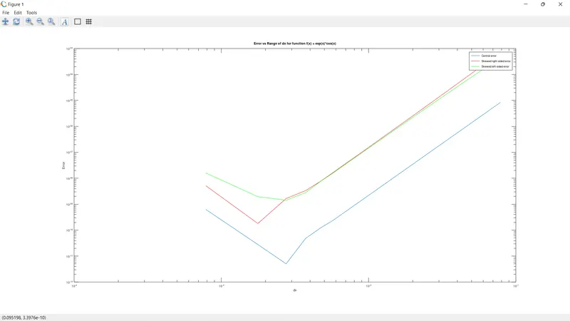
• The above graph compares the error calculated for the function f(x) = exp(x) * cos(x) double derivative for the central, skewed right – side and skewed – left side differencing schemes.
• It can be concluded that the error for right-side and left–side skewed differencing are similar.
• Whereas, the error for central differencing is low as compared to others.
• Therefore, central differencing is better than other schemes because it uses information from both sides from the point of consideration to provide approximative and accurate values.

The central differencing scheme has advantages as it is easy to understand and implement, and its convergence rate is faster than other finite differencing methods.

WHY A SKEWED SCHEME IS USEFUL? WHAT CAN A SKEWED SCHEME DO THAT A CD SCHEME CAN NOT?

Skewness refers to a distortion or asymmetry that deviates from the normal distortion in a set of data. The skewed scheme method considers information from either ( left or right ) side node of the considered patch and provides numerical solutions to differential equations. When data for the grid points is only available from one side of the domain and high order approximations are required, we compute using skewed schemes, such as depicted in the scenario. The central difference approximation scheme is less likely to be considered in calculating a function at the boundary of a domain. This is where skewed schemes are useful.