Week 1- Mixing Tee

Aim:

To perform a steady state simulation to analyse the mixing effectiveness in a Tee joint when two streams of hot (@ 36degC) and cold jet (@19deg C) mixes.

Also to identify the variation of results between using the K-epsilon and K-omega methods.

To calculate the cell count, average outlet temperature, number of iterations to converge, velocity and temperature contour among varying pipe length, momentum ratio, velocity of jets etc.

Introduction:

Mixing Tee is a 'T' shaped duct which is used in Heating Ventilation Airconditioning (HVAC) applications, which facilitates efficient mixing of two streams of varying temperature.

The duct part model here has a circular cross section on both inlet and outlet. The cold air is passed from the y-axis oriented inlet, and hot air is passed through the x-axis oriented inlet. The two streams are analysed at varying velocity of momentum ratio 2 and 4.

The analysis is further classified among two varying length of the Tee ducts.

Also efficiency of k-epsilon and k-omega viscosity models are also analysed.

Procedure:

The procedure is explained for 1 example case as short Tee.

The simulation is done with fluent module in Ansys workbench

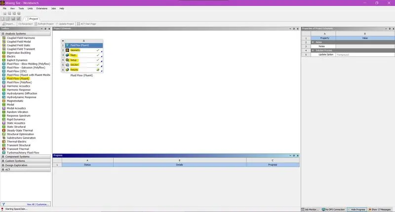
All the pre-processing, simulation and post processing stages are done in 5 steps as shown in the above image

Step 1 - Setting geometry

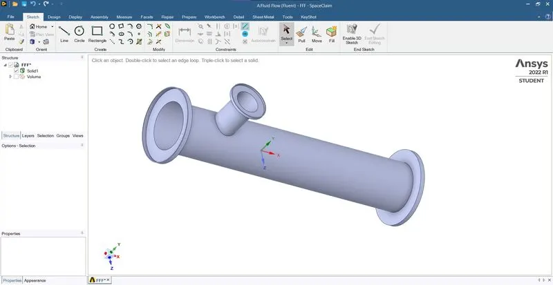
This is done in Space Claim component.

Fluid volume extraction and selection of geometry for physics is done

Short Tee part model: part model is loaded from Solid Works.

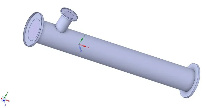
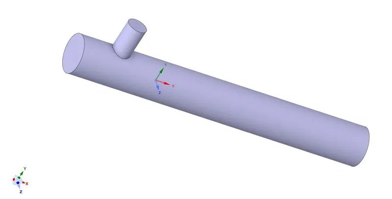
Long Tee part model:

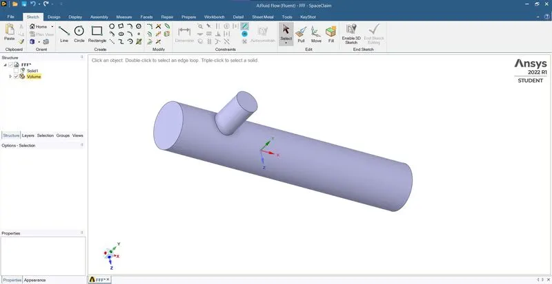
Selecting the fluid volume: Fluid volume is extracted to do simulation only for the fluid flow

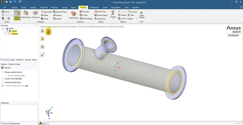
Extracted volume: Fluid volume is extracted and made into a separate volume

Long Tee part model:

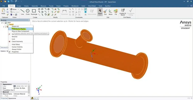
selection of geometry for physics: The geometry which is not going to be used in simulation is suppressed for physics

Step 2.Setting up the mesh

It is done in the mesh component

Mesh generation, setting up inlet, outlet, walls are done in this step

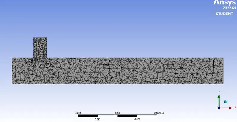
Generated mesh:

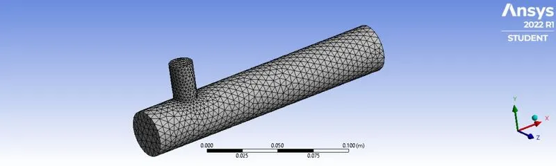
Analysis of mesh using section plane:

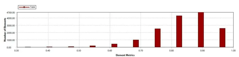
Mesh metrics:

Selection of faces to fix boundary conditions: Face selection tool is used to select different faces

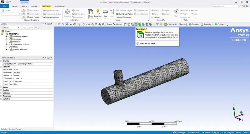
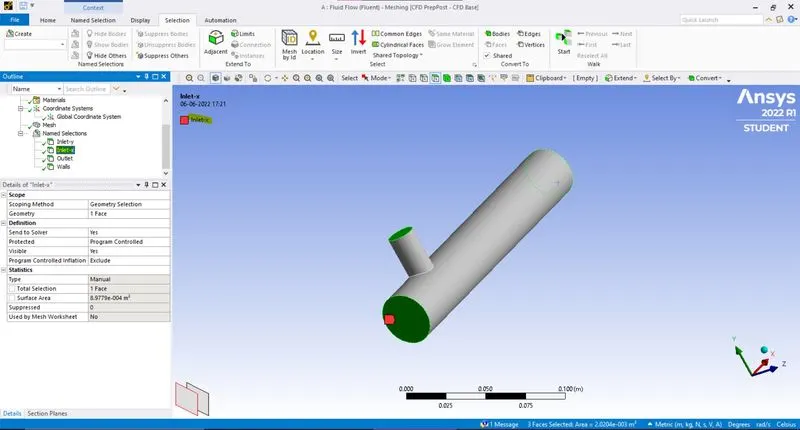
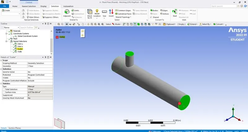
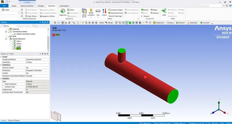
Named selection option is used to define the boundaries to the system

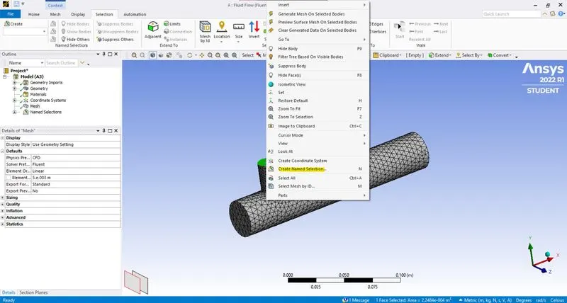
Inlet-y defined:

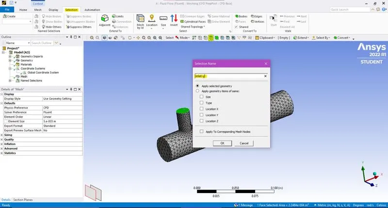
Selected Inlet-y:

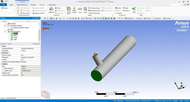
Selected Inlet-x:

Selected outlet:

Selected walls:

Step 3.Simulation setup

This is done Ansys Fluent component.

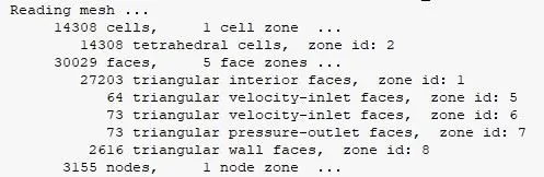
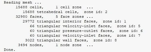
Genareted mesh details from console:

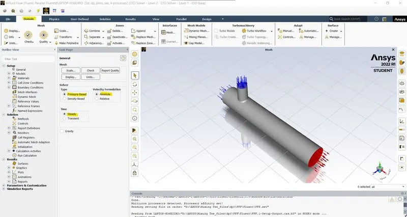
Setting up domain: In domain, Pressure based type, Absolute velocity formation, Steady time simulation are selected

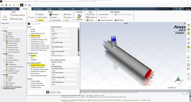
Setting up physics, K-Epsilon model Standard is selected

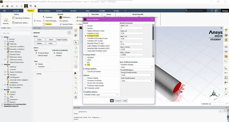
K-omega SST model is also be set up for another case:

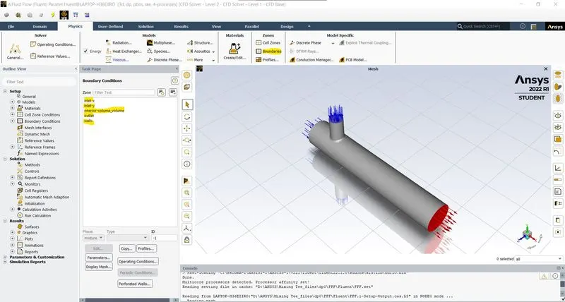
Setting up boundary conditions:

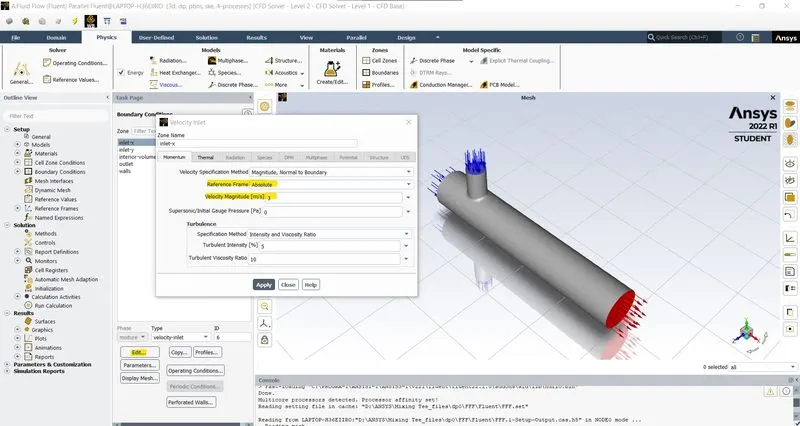
Setting up inlet-x velocity:

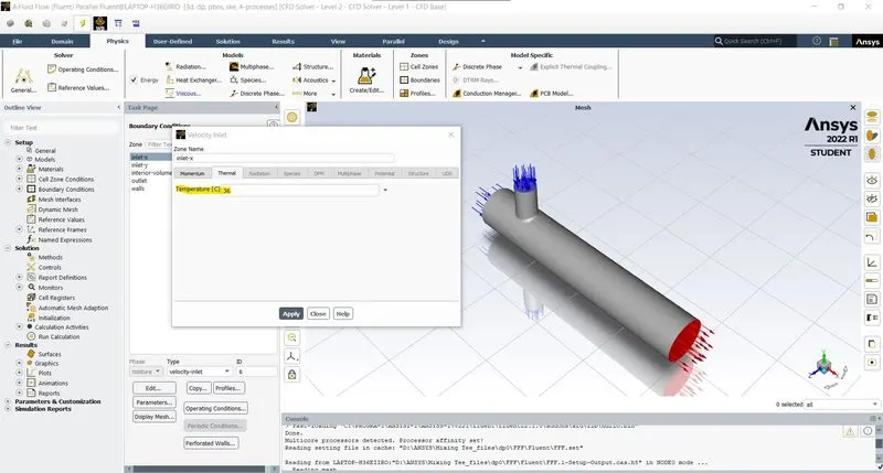
Setting up inlet-x temperature:

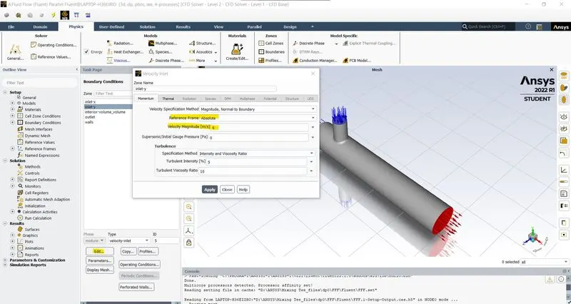
Setting up inlet-y:

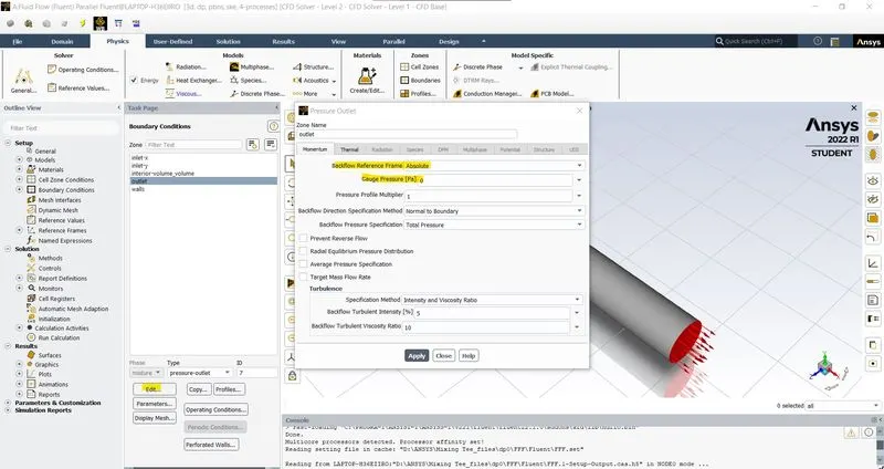
Setting outlet:

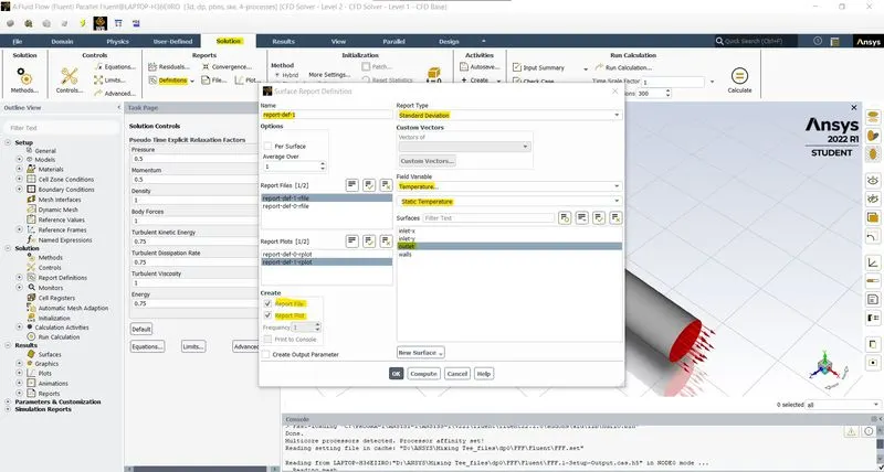
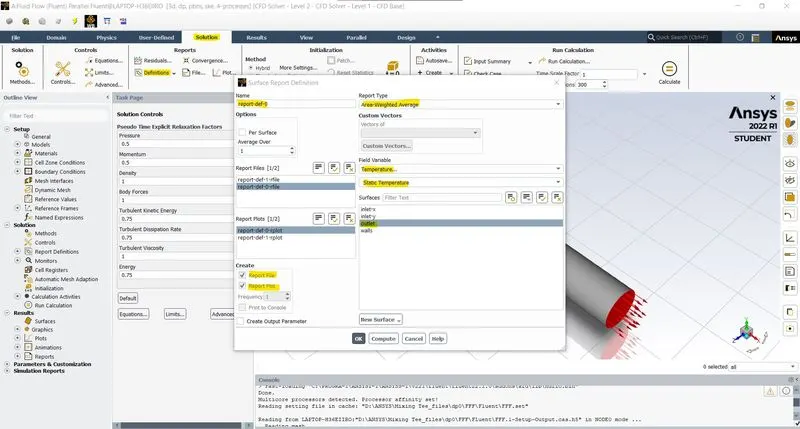
Defining variables for plots and reports of the result:

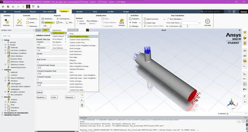
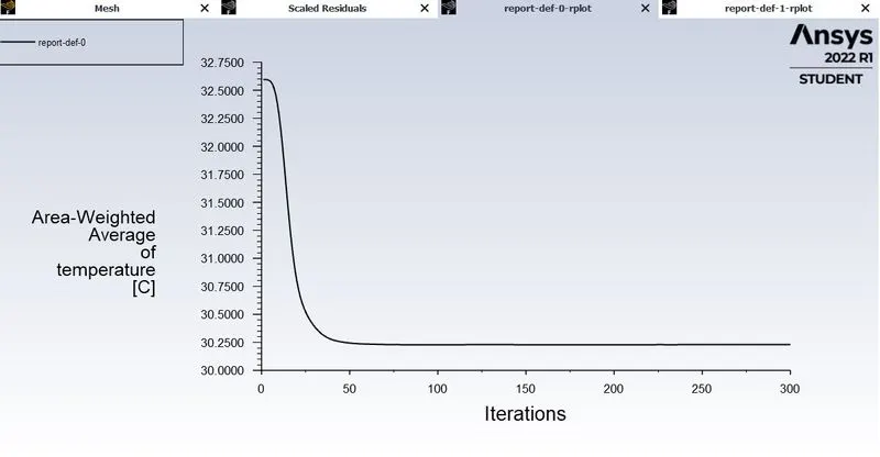
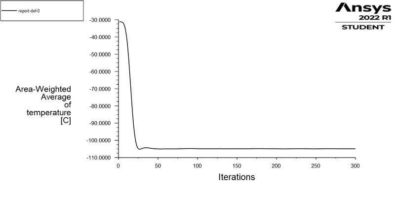
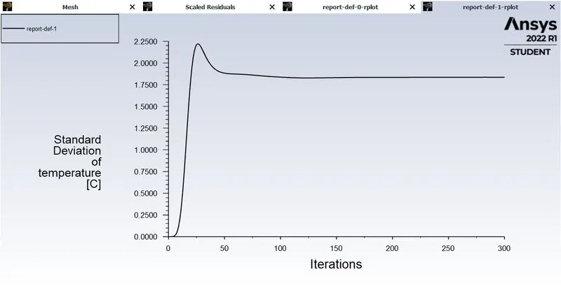
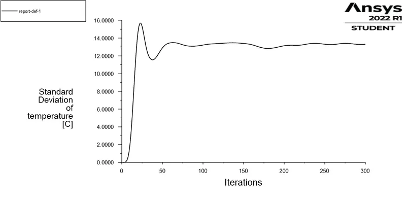
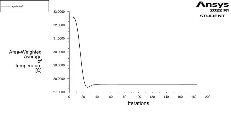
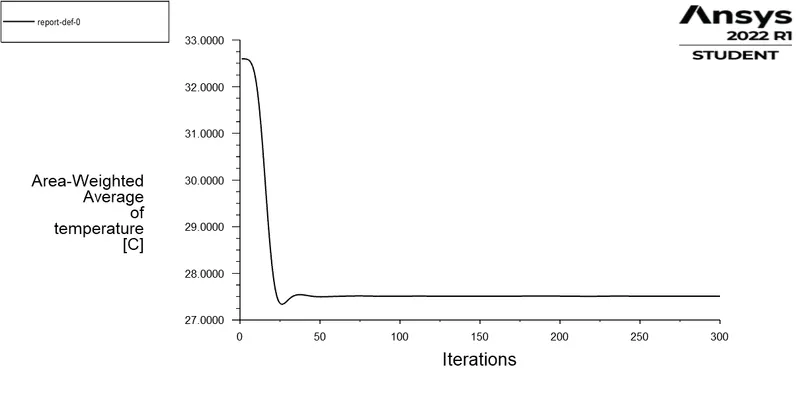
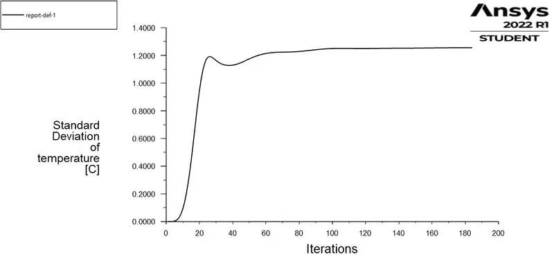
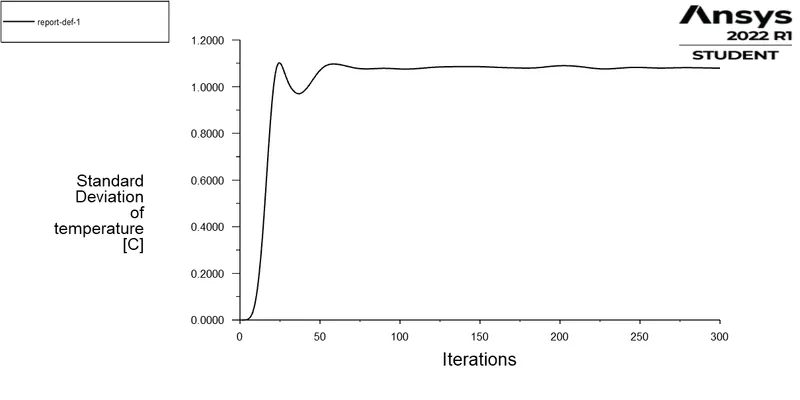
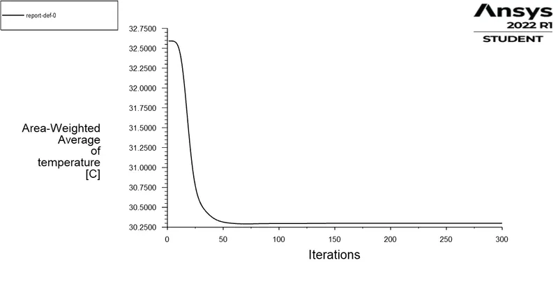
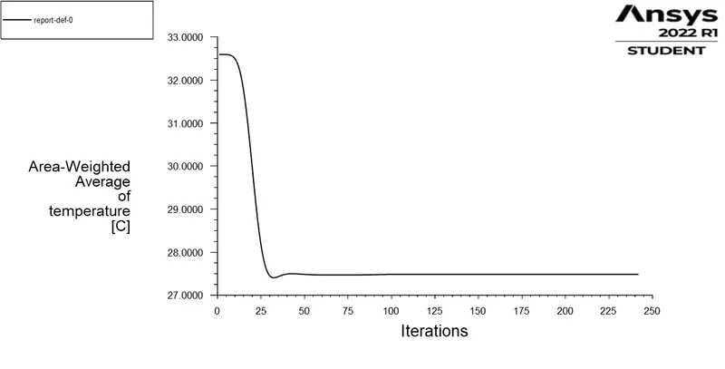
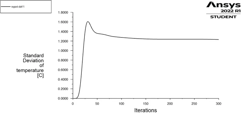
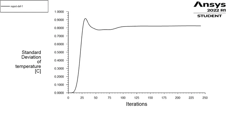
Two report and plot are defined, one for area-weighted average and the other for standard deviation of temperature.

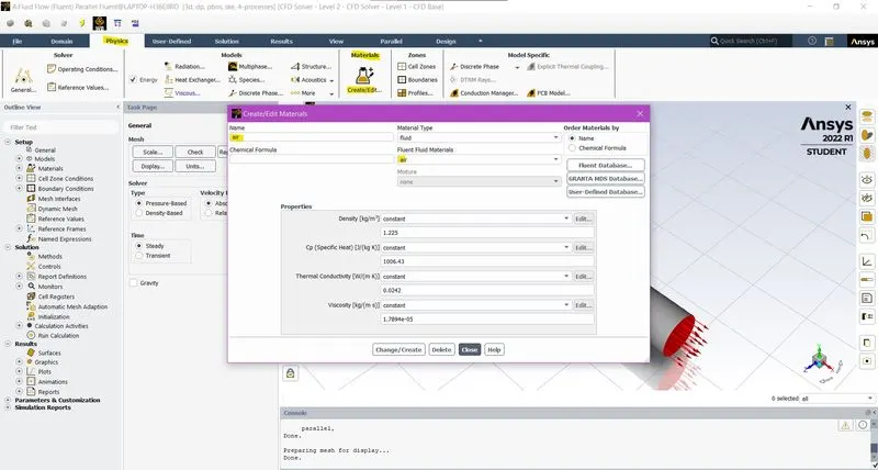
Material definition, the fluid is given as air:

Step 4.Solution simulation

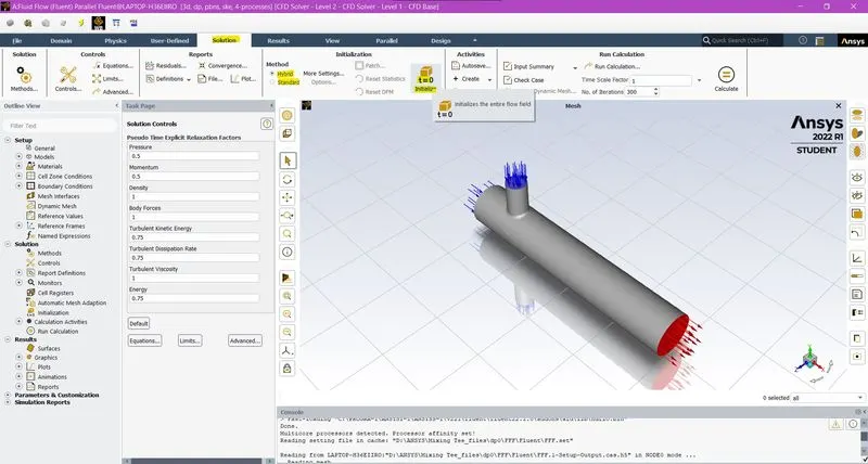
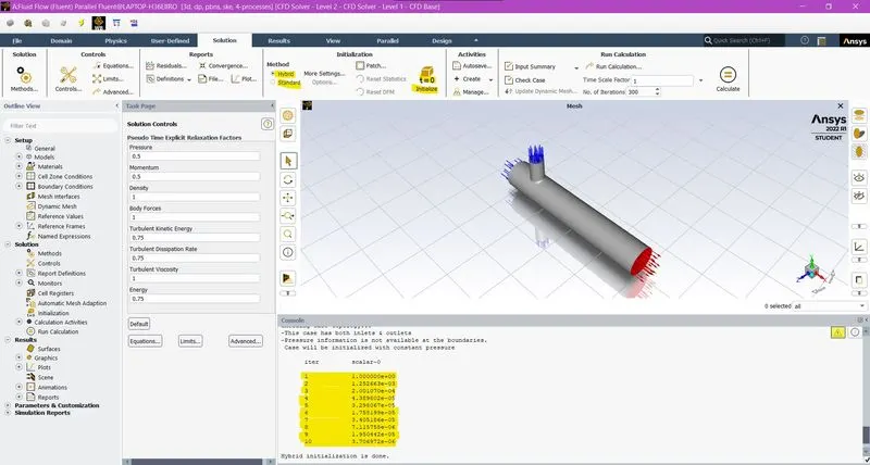
Initialization is done with hybrid method:

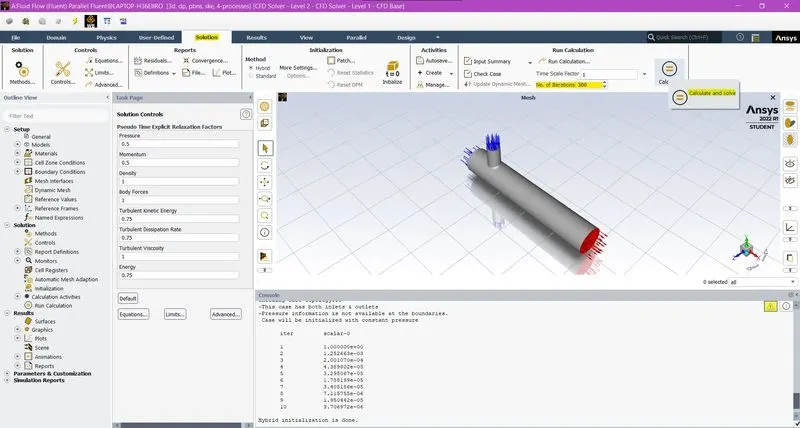
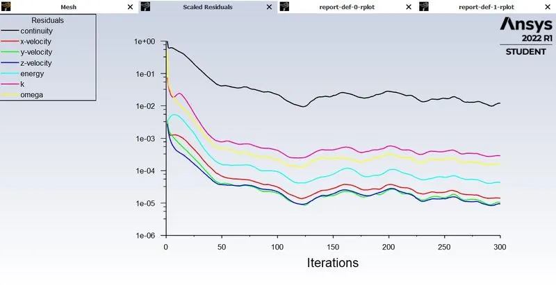
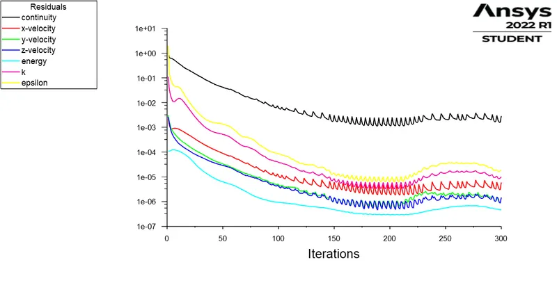
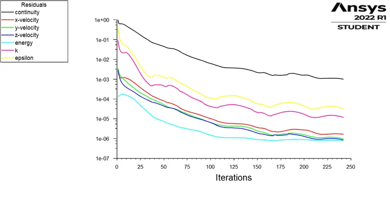
Simulation is run using the calculate command, for 300 iterations:

Step 5.Post processing the results

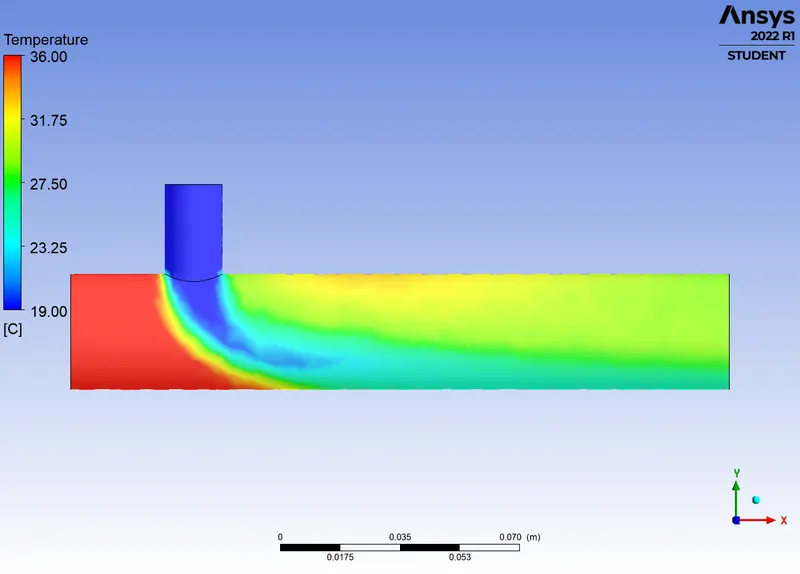
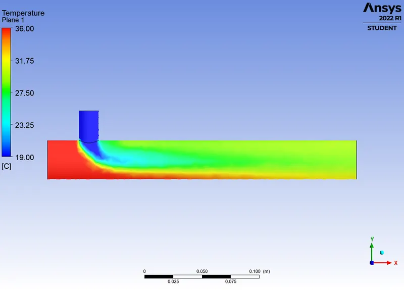
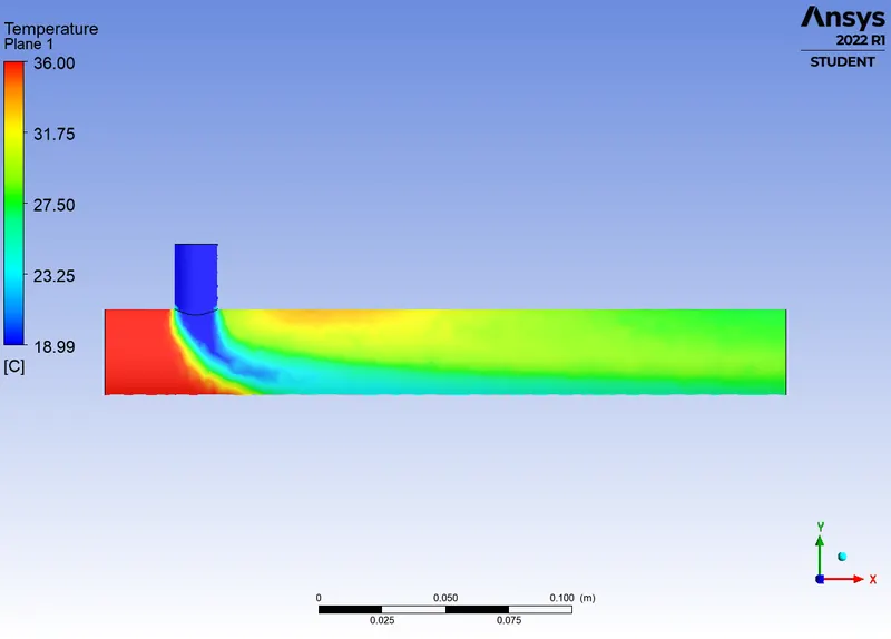
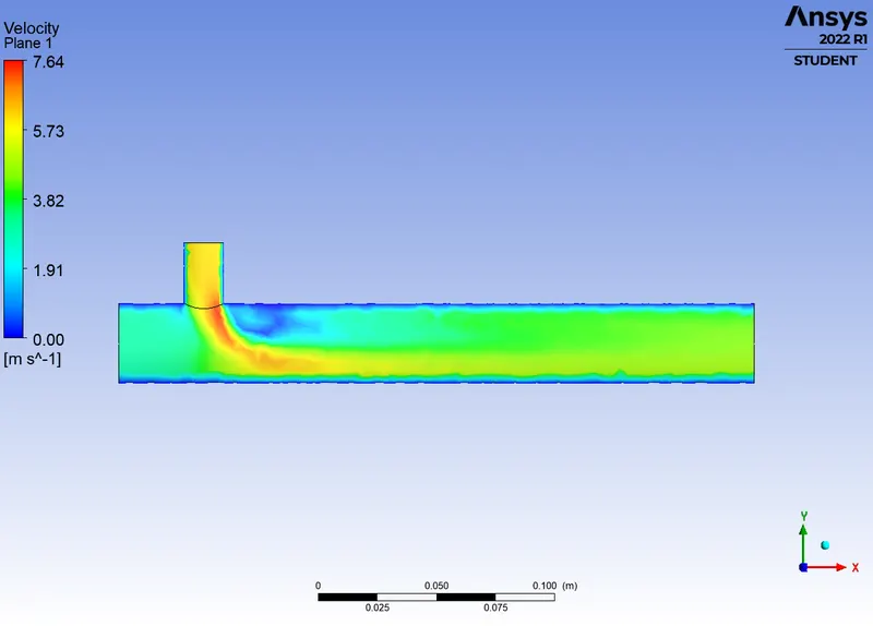
The result reports and plots are discussed below for each case.

Results:

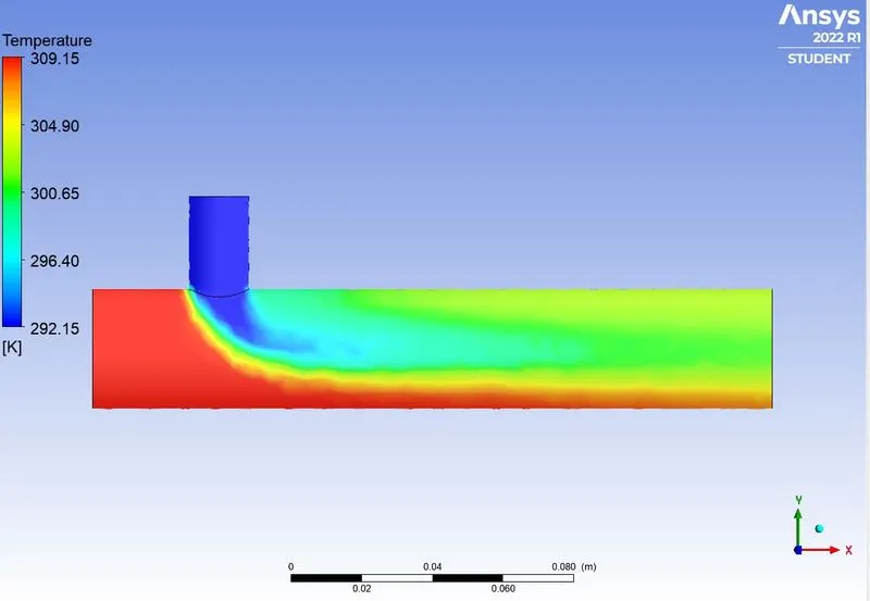
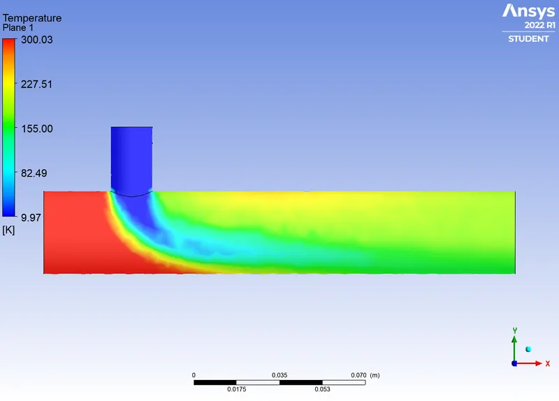
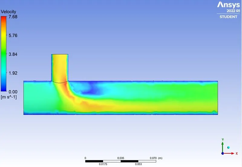
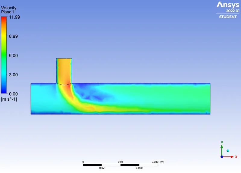
Case 1:

K-epsilon vs K-omega

Short Tee

Inlet velocity of hot air: 3m/s

Inlet velocity of cold air: 6m/s (From Momentum ratio = 2)

Inlet temperature of hot air: `36^o C`

Inlet temperature of cold air:`19^o C`

Mesh data:

K-epsilon model	K-omega model

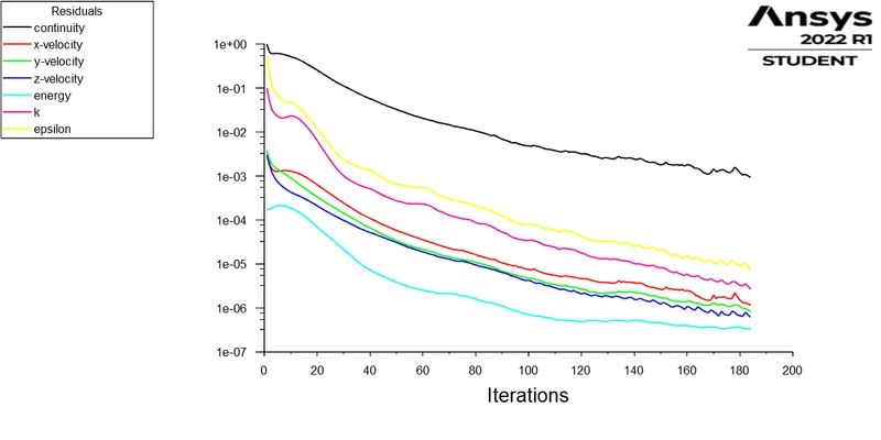
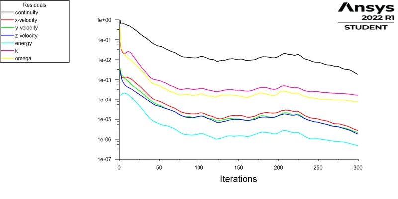
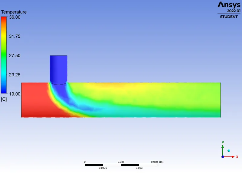
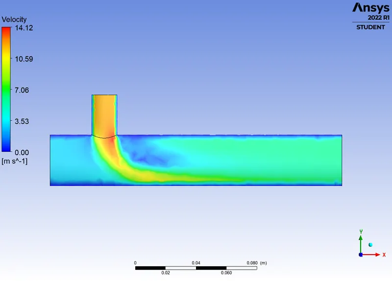
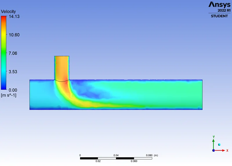
Case -2:

K-epsilon vs K-omega

Short Tee

Inlet velocity of hot air: 3m/s

Inlet velocity of cold air: 12m/s (From Momentum ratio = 4)

Inlet temperature of hot air: `36^o C`

Inlet temperature of cold air:`19^o C`

Mesh data:

K-epsilon model	K-omega model

Case -3:

K-epsilon

Long Tee

Mesh data:

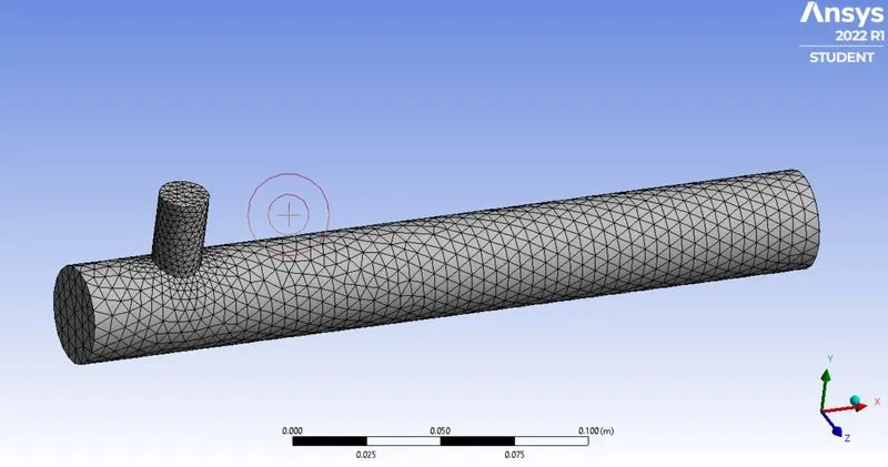
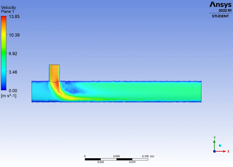
Inlet velocity of hot air: 3m/s

Inlet temperature of hot air: `36^o C`

Inlet temperature of cold air:`19^o C`

Inlet velocity of cold air = 6 m/s (Momentum ratio=2)	Inlet velocity of cold air = 12m/s (Momentum ratio=4)

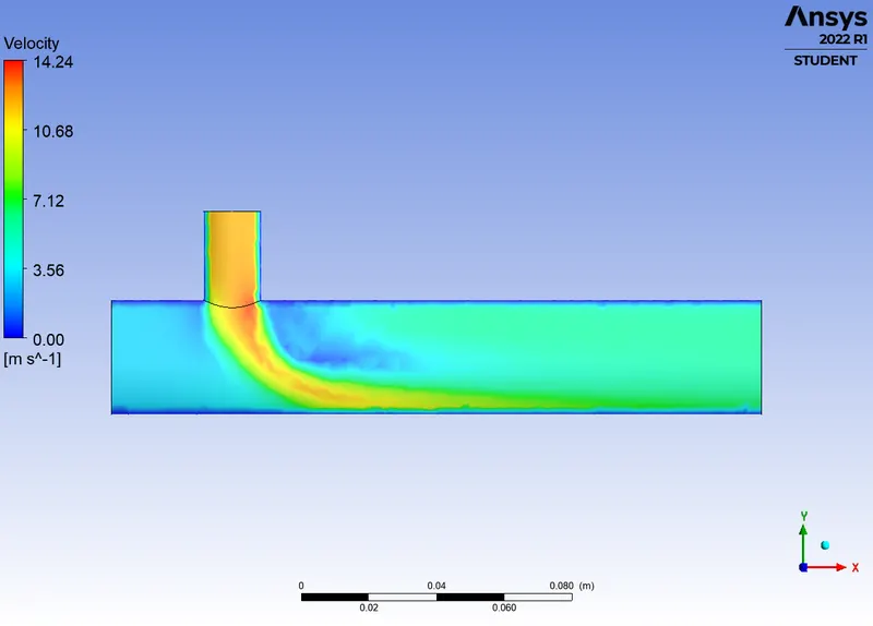
Case -4 Mesh Refinement:

K-epsilon

Short Tee

Inlet velocity of hot air: 3m/s

Inlet velocity of cold air: 12m/s (From Momentum ratio = 4)

Inlet temperature of hot air: `36^o C`

Inlet temperature of cold air:`19^o C`

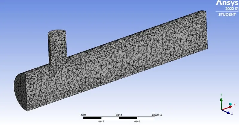
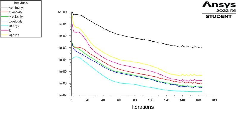
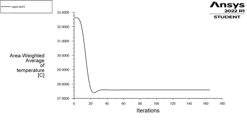
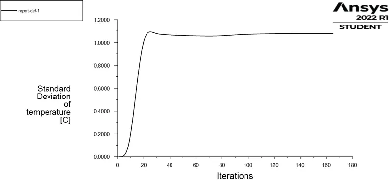
Mesh element size is given as 0.003.

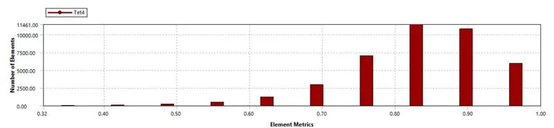
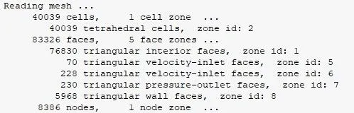
Mesh data:

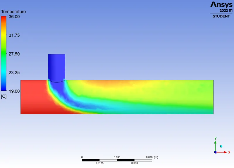
Inference:

Quantities	units	Short Tee (MR = 2) K-e	Short Tee (MR=2) K-w	Short Tee (MR = 2) K-e	Short Tee (MR=4) K-w	Long Tee (MR=2) K-e	Long Tee (MR=4) K-e	Short Tee MR=2, K-e, e=0.003
Number of cells	nos.	14308	14308	14308	14308	15688	15688	40039
Average outlet temperature	deg C	27	28	29	29	28	28	28
Average outlet velocity	m/s	4	5	6	6	4	5	5
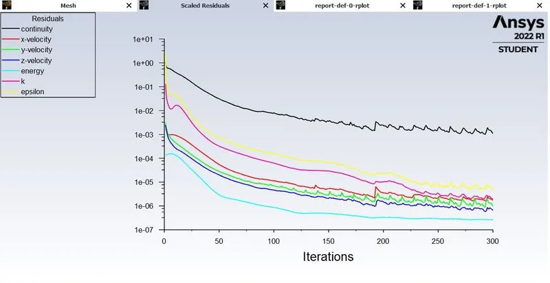
Number of iterations to converge	nos.	50	40	30	40	50	35	35

Conclusion:

From the above analysis, it is noted that K-epsilon model can predict flow far from boundaries and K-omega model can predict flow near the walls.

In case of momentum ratio, a higher momentum ratio gives better mixing efficiency at outlet

In comparison between the length of the Tees, short tee provide better mixing of streams

Also when the number of cells are many, it takes much time to converge

Based on the inferences for a fully efficient mixing tee, the length is to be short with momentum ratio high and the simulation to be performed with K-epsilon and coarse mesh with optimum number of cells.