Week 1- Mixing Tee

Objective :

To simulate the flow of air through mixing tee and understand the effect of the length of the pipe and momentum ratio of velocity for mixing the air by using two different types of pipe i.e short pipe and long pipe.

About

In industrial process engineering, mixing is a unit operations that involves the manipulation of a heterogeneous physical system with the intent to make it more homoegenous. Mixing is performed to allow heat and mass transfer to occur between one or more streams, components or phases. Modern industrial processing almost always involves some form of mixing. mixing tee is a type of mixing mechanism. Mixing Tees utilizes a specifically engineering internal geometry to efficiently mix two fluid streams into one combined stream. Mixing tees are widely used in the petrochemical, HVAC industry etc. In which two fluids streams with different physical and chemical properties mix together.

Hot air flowing in the main pipe is mixed with cold air flowing through a tee. The standard deviation of temperature is computed to quantify the degree of mixing. The velocity and temperature fields are also computed. The effect of the mesh size, turbulance model on results were examined.

For this, we have created two versions of mixing tee. one of them is longer than the other.

It is set up as steady-state simulation to compare the mixing effectiveness when hot inlet temperature is 36 degree celsius & cold inlet at 19 degree celsius.

1.Case 1

• Short mixing tee with a hot inlet velocity of 3m/s.
• Momentum ratio of 2,4.

2. Case 2

• Long mixing tee with a hot inlet velocity of 3m/s.
• Momentum ratio of 2,4.

Momentum ratio is defined as the ratio of velocity at the cold inlet to the velocity at the hot inlet.

`Momentum ratio = V_c/V_h`

Case setup -

CAD cleanup/Pre-processing-SpaceClaim

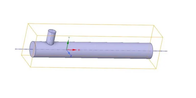
The CAD model is imported imported into the SpaceClaim to extract the flow volume field from the model. The extracted volume is shown below :

Mesh

The boundary names are applied in the section and mesh is generated.

Setup

In this section, we apply different boudary conditions like inlet, outlet boundary conditions. Turbulence models are set up like K-epsilon or K-omega for solving the turbulent mixing of air. The number of iteratin set in this section.

CFD-Postprocessing

Post-processing is carried in this section in which different contours are setup to visualize the properties ( such as temperature, velocity etc.) for which simulation is run.

BASELINE SIMULATION -

For inlett velocity of 3m/s and momentum ratio of 2

default mesh - 0.010219m

PROCEDURE -

There are three major steps to perform any type of simulation as follows pre-processor - it includes geometry clean up and generate besh quality mesh. Solving includes applying boundary conditions, initialize and convergence. Last step is post processor which includes generate plots,contours,vectors to analyze results. In this study we are going to follow all three steps to find out effectiveness of mixing tee. The following steps to be followed -

Here for solving we used Ansys fluent.

There are basically 5 lists of steps such as Geometry, Mesh, Setup, Solution and Results.

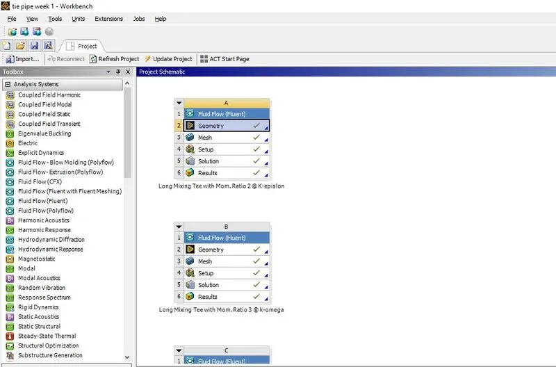
1. Firstly, i am going to start with Geometry preparation in SpaceClaim. Spaceclaim is very nice cadmodeling software that can be used to prepare cad model for simulation setup it could be for FEA or it could be for CFD. Once's this is loaded, click on file then open and going to navigate where the geometry file have been stored.

2. So firstly, i a going to be selecting Long mixing Tee file geometry and click on open,its import mixing tee model. It will redirect to Spaceclaim, Ansys's geometry model manipulator.

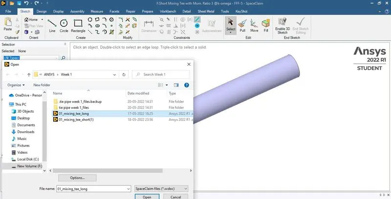
3.Now the geometry has loaded, this is what we called as mixing tee. In this particular case i am interested to performing the flow simulation. Im here extracting the fluid volume. How to extract volume, well going to prepare there is an option called Volume extracted, i am gong to use the select edges method. Here i am selected the follwing three edge and click on click on green mark.

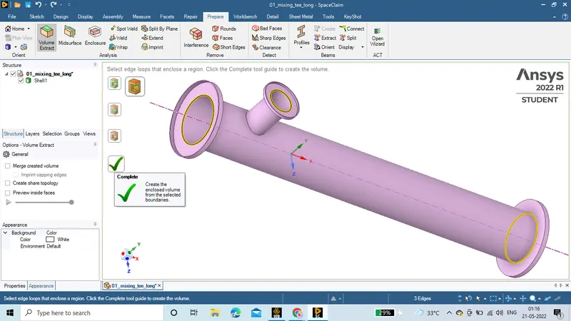
4. Now i can see that a new object is added to my tee and i am going to hide a solid component and whatever i have left that is my fluid volume.

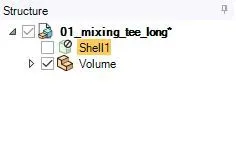
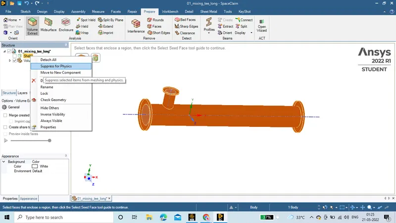
5. So, in order to ensure that the solid component is not going to be loaded during meshing process. i was slected shell and do suppress for physics. so there is small symbol on the solid which shows that it has been suppressed.

6. Now, i am going to close this particular model, thing are saved automatically.

MESH : -

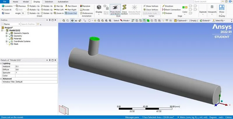
7. Here i am going to name the boundaries that we have so that we can add the appropriate meshing and also when we applying the boundary conditions we can select the boundaries that we created.

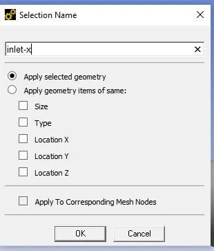
Press ctrl+ F for face selection and press N for name selection and provide particular name for these faces such as 'inlet-x' for the hot fluid enter into the system and 'inlet-y' for the cold fluid enter into the system and outlet for fluid exiting from the tee. select the two surfaces and give it name as 'walls'.

Here i am gong to provide the value of element size is '2' in order to get finer mesh. and update the mesh by clicking on mesh button.

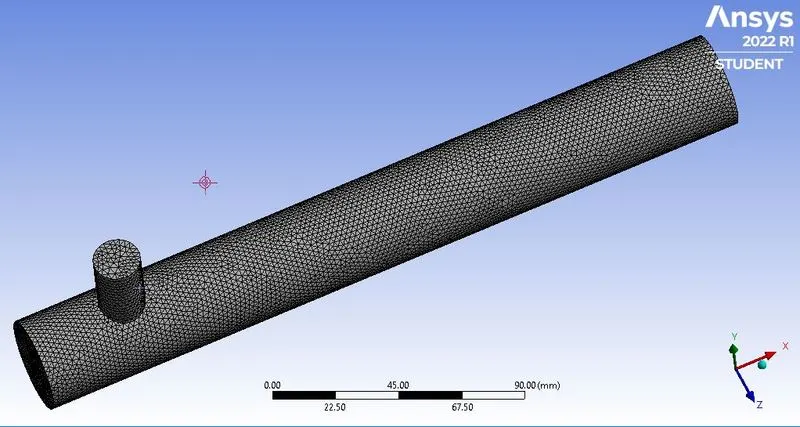
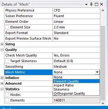
8. So this is computational Mesh. So in this particular Case i am going to click on 'Quality' and select Element quality in mesh metric.

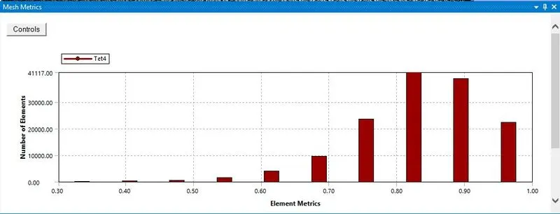
when i do this i immidately get animate which look histogram.On the x-axis we have Element matrix or the element quality and on the y-axis we have number of elements. we can see here minimum and maximum quality.

SETUP : -

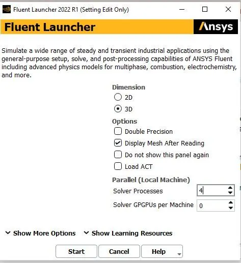
9. Click on 'Setup' and its going to open 'ansys fluent' , i am going to doing simulation here with 4 processor.

10.Here we have 'console' which contain important information regarding simulation about geometry and mesh are presented, if there any error it shown up here. some errors are shown up in the dialogue boxes but if its run time error meaning if the error is generating as simulation runs its going to appear here.

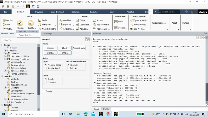
And we have 'Graphics' here where we can see our simulation. In this the navigation is bit more different.

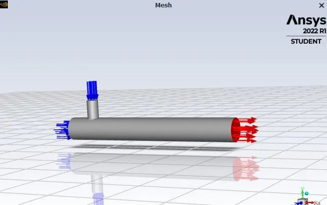
Firstly, we need to check the mesh quality so we can see print everything there is no any kind of warning messages or errors that typically means mesh is OK.

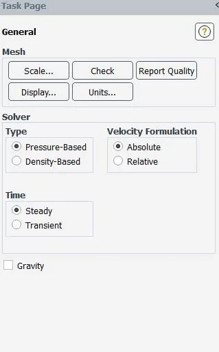
Now, move to 'physics' bar so in this particular case i am goingto use 'steady'state solver and for really small mac number flows its good to use 'Pressure-Based' solver and for Velocity formulation i am going to use 'Absolute' option.

11. Now we are interesed in solving 'Temperature' so we will be using 'Energy' equation as well and in this particular case the flow can be turbulent so i am going to select the 'Turbulent' model and i am using here 'K-epislon' turbulence model and used upgrade version of its which is called as 'Realizable' k-epislon model with standard wall function .

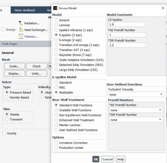
These k-epislon and k-omega are called as RANS-based tubulent model or'Reynold Average based Navier Stocks' turbulence model .

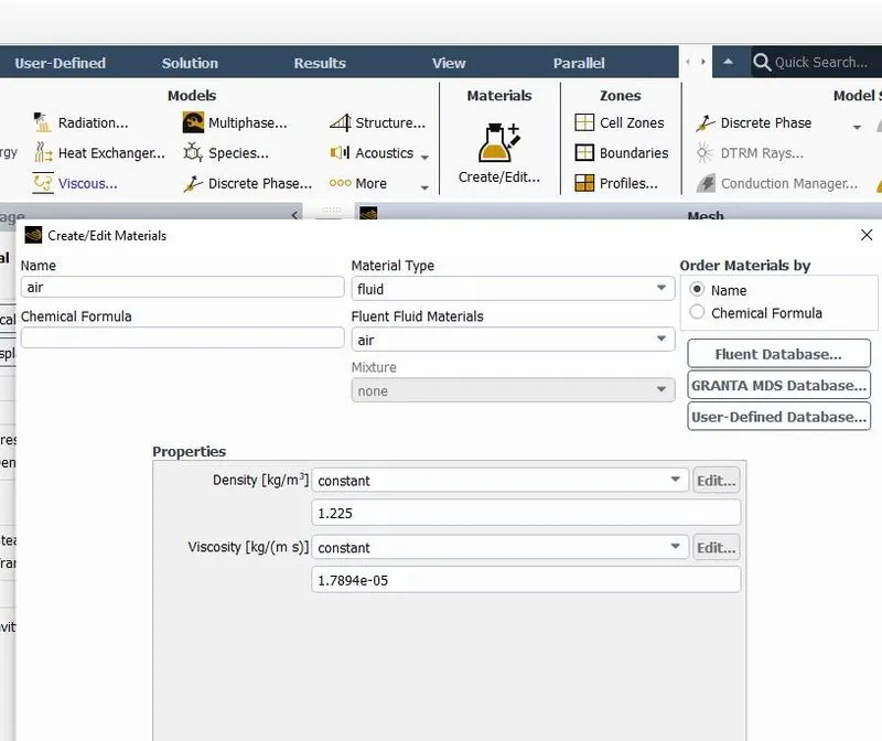
Next i am going to add material, just click on materials as we can see that 'air' is the working fluid here .

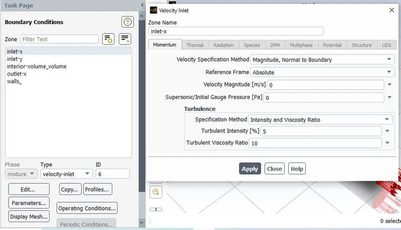
12. Then, we are going to assign the boundary conditions so go to 'Zones' first select 'Cell zones and next select 'boundaries' and let's start with 'inlet-x' and we can see the Type is automatically select to 'velocity-inlet' and click on edit and provide the value of inlet velociy face which is 3m/s and incoming inlet value of temperature i.e 19 degree C. In addition to it, for y-axis the value of cold inlet velocity is 6m/s and the value of incoming air is 36 degree C. Also, for 'oulet' boundary condition when i click on it i can see that at the outlet the pressure is 0 now remember this is gauge pressure.

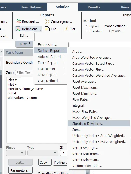
13. So in order to understand the effectiveness of mixing problems one thing is engineers look at is surface 'standard deviation' This time click on 'Definition' create a new report and see standard deviation here, select temperature as Field variable and outlet and click on create a report.

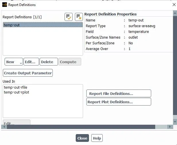
we can see the report definition file in the definition tab go to definition and click on edit here we can se the 'reports' what we are created before.

14.Once we setup the initial conditions, boundary conditions and material properties the thing we need to do is initialize the Solution. So for performing CFD analysis we are solving for velocity, pressure, temperature and other variables.

15. Now i am going to click on to the initialize button we are using hybrid initializing process used as a potential fluid solver to compute an aapproximate value of velocity and pressure. So as we can see in the console the 10 iteration is done .Now we are ready to Run thesolver. Generally, i am going to run it for a 300 iteration and hit calculate. when i do this i can automatically see lot of plots. The first plot is looking at the 'Area-weighted Average of temperature(C) Vs no. of iteration and second plot is Standard deviation of temperature Vs no. of iteration and we can also see something called 'Residuals' , so what it does mean when we solving bunch of CFD equations and thesen are partial differential equation ,any partial equation or governing equation is going to be on the form soem function is equal to be a zero when we solve these function/equation on a computer we apply some kind of approximations that is what we called as numerical discretization which in this case is called 'finite volume method' . so we use the FVM approach to dicretize the partial differential equation and we solve it. when we actually solve the function it might not evaluate to 0 , it miggt evaluate to something really really small something like 1e-5. So in this particular case what we called as residuals, so the number of iteration continue what we can seen here is the function is being calculate and its very very close to 0 except certain cases like continuity like 1e-4 which is very small number so with that we simulation is completed.

16.So, now we need to Post-process the 'results' and i am going to back in workbench and click on 'Results'.Now i am enable all the components and uncheck inlet and outlet.

17. Now i am applying transprancy to my model with the help of rendering .

18. Let's go to insert -->location--->plane and give a name it as 'plane1' . we can see that a XY plane in the middle of the model.

19. Now i am go back to my plan double click on it and color this by 'variable' and choose the variable as 'Temperature' and apply. Now we can see that a model with variable colors.

20. Go to details of plane1 choose color bar and give the color range from 10 degree C to 25 degree C and apply and legends going to be changed

21. Go to default legend view1, here go to Apprerance and provide fix point notation upto 2 decimal places and click on apply.

There are so many intersting thing can be observed here the mixing process is primarily determined by the velocity of the incoming jet and we can use different values of momentum ratio

which basically means ratios of velocity at inlet-x to inlet-y currently i can seen that the velocity at inlet-x is 25 and inlet-y is 10 . we are basically examine the mixing process by applying different momentum ratio. The solution here become diffuse and that's because of our mesh resolution.

Repeat the same procedure for cold fluid coming,velocity 6m/s, temperature 19 c.

We want to generate temperature report of outlet and we want standard deviation of temperature also. Go to solution tab and definition and select are weighted average. In the opened menu select temperature as field variable. Similarly select standard deviation in definition menu.

22. Now click on initialization to calculate approximate values of velocity and temperature.

5. Results -

Case 1 - In this short mixing tee is used, which was mixing two fluid with temperature 36 and 19 degree C. Velocity of hot fluid was 3m/s and cold fluid was 6m/s. we used two different turbulent solvers for it first was realized k-epsilon and second was k-omega SST.

In this case k-epsilonis giving better results because the solution was converged after few iterations, whereas after using k-omega model solution was not converged . k-omega is preferred in studying fluid behaviour near wall, but here it is not the case. So, k-epsilon model is recommended to study of fluid far from wall i.e flow region.

# Plots and contours from k-epsilon model for short mixing tee @ momentum ratio = 2

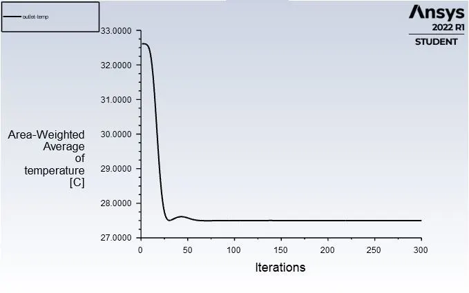
Fig. Average Temperature vs Iterations

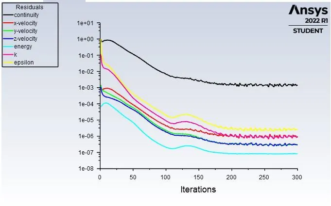
Fig. Residuals

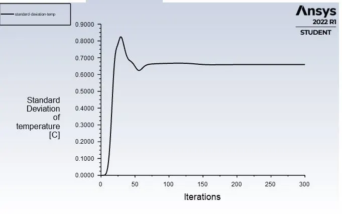
Fig. Standard Deviation of Temperature vs Iterations

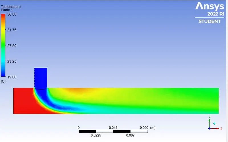
Fig. Temperature Contour along the length of the pipe

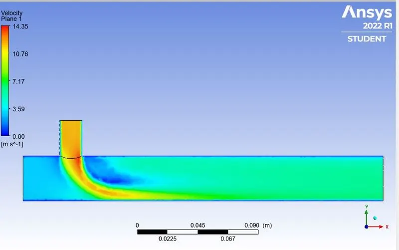
Fig. Velocity Contour along the length of the pipe

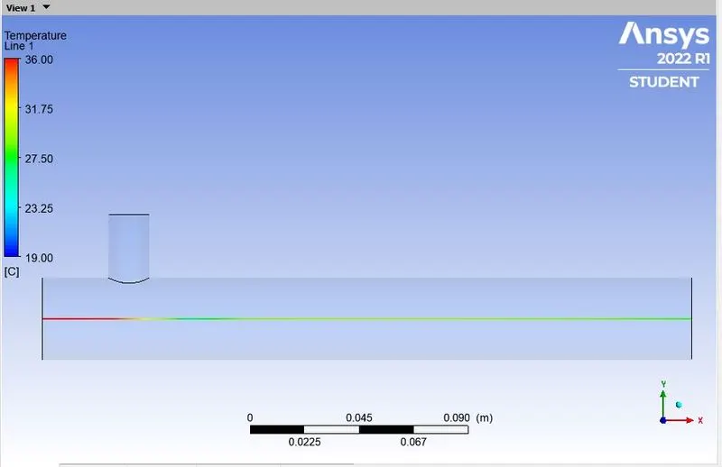
Fig. Temperature Line plot along the length of the pipe

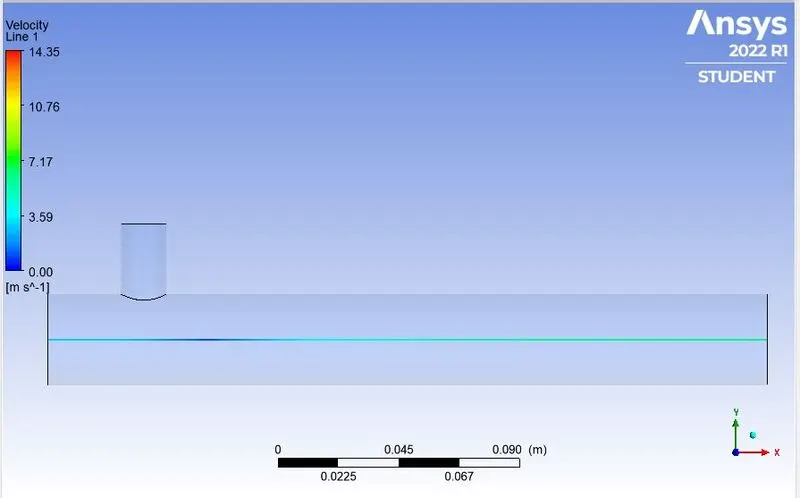
Fig. Velocity Line plot along the length of the pipe

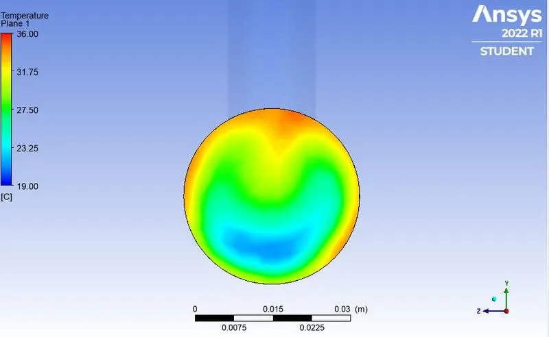
Fig. Temperature plot along the length of the pipe

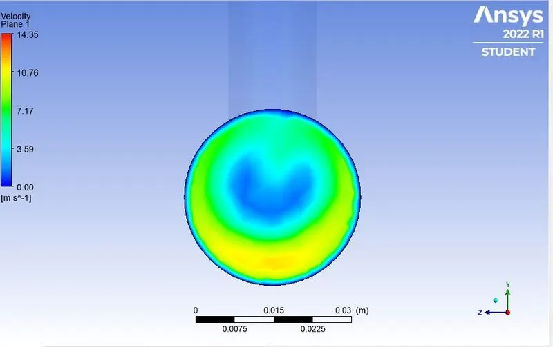
Fig. Velocity plot along the length of the pipe

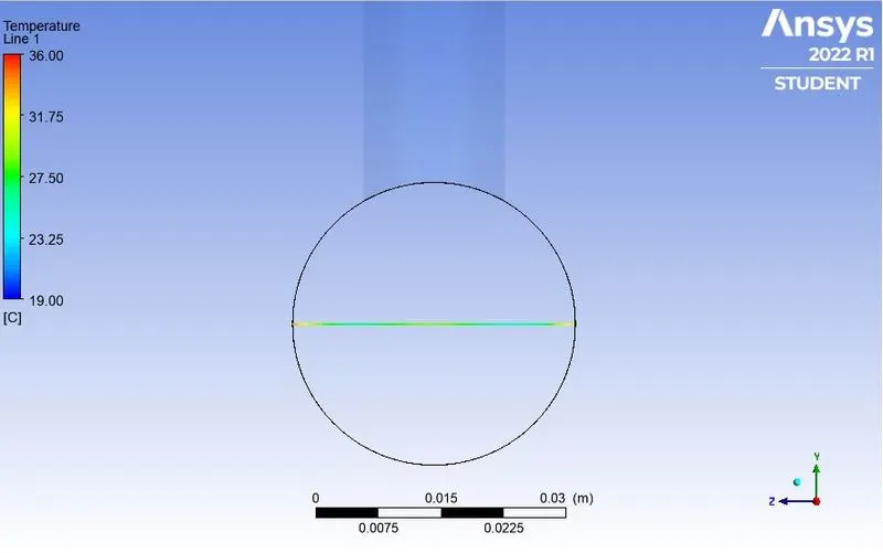
Fig. Temperature Line plot across the length of the pipe

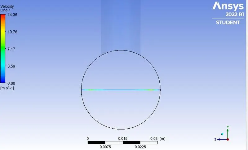
Fig. Velocity Line plot across the length of the pipe

# Plots and contours from k-epsilon model for short mixing tee @ momentum ratio = 4

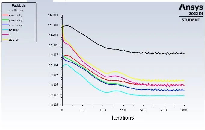
Fig. Residuals

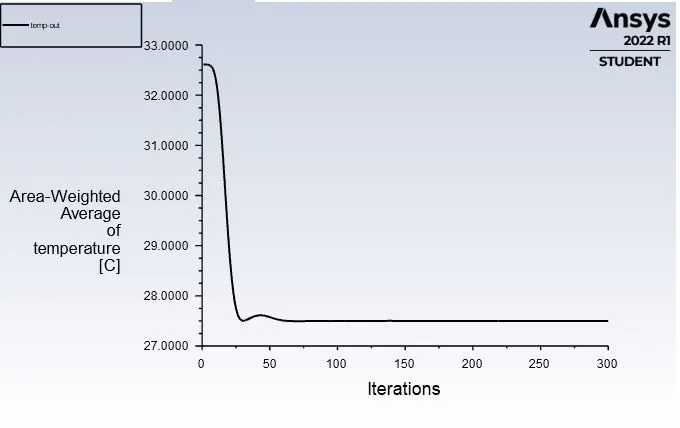
Fig. Average Temperature vs Iterations

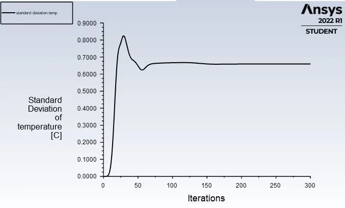
Fig. Standard Deviation of Temperature vs Iterations

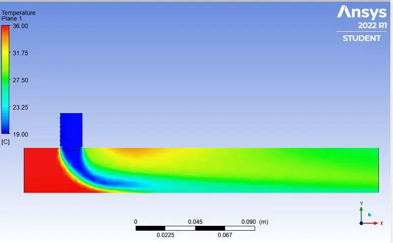
Fig. Temperature Contour along the length of the pipe

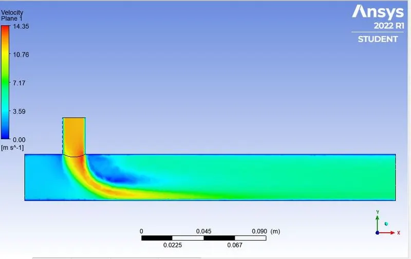
Fig. Velocity Contour along the length of the pipe

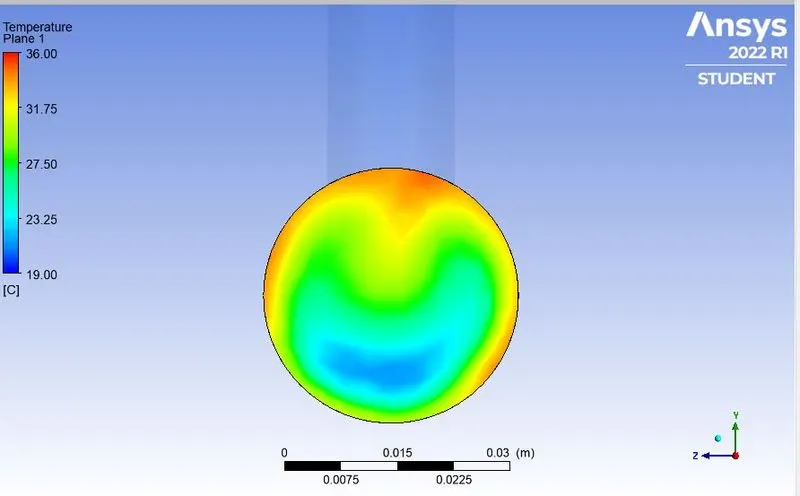
Fig. Temperature plot across the length of the pipe

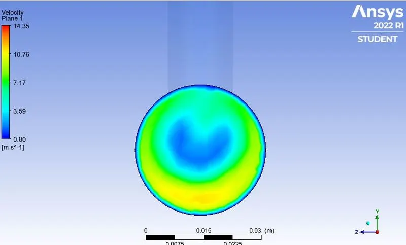
Fig. Velocity plot across the length of the pipe

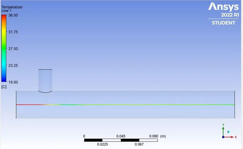
Fig. Temperature Line plot along the length of the pipe

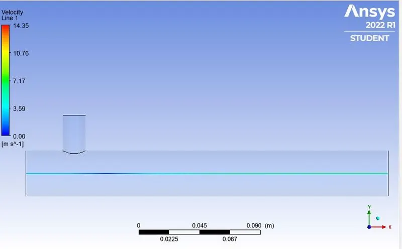
Fig. Velocity Line plot along the length of the pipe

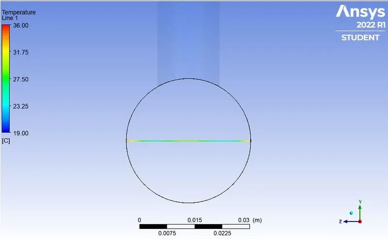
Fig. Temperature Line plot across the length of the pipe

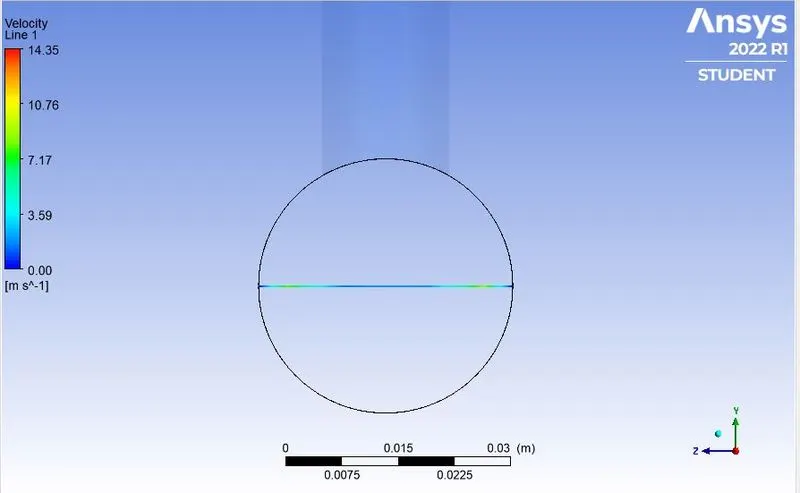
Fig. Velocity Line plot across the length of the pipe

# Plots and contours from k-omega model for short mixing tee @ momentum ratio = 2

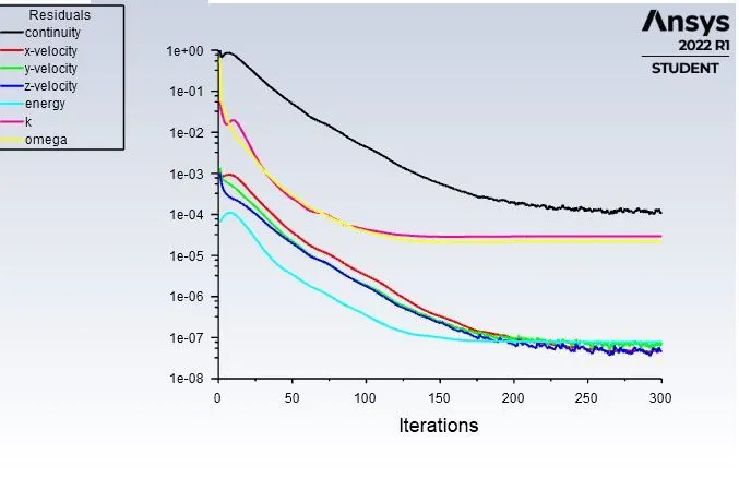
Fig. Residuals

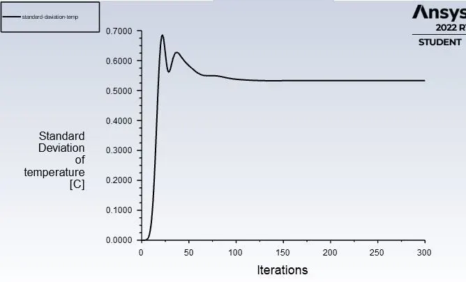
Fig. Standard Deviation of Temperature vs Iterations

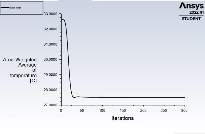
Fig. Average Temperature vs Iterations

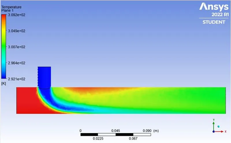
Fig. Temperature Contour along the length of the pipe

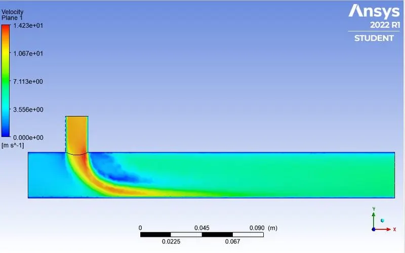
Fig. Velocity Contour along the length of the pipe

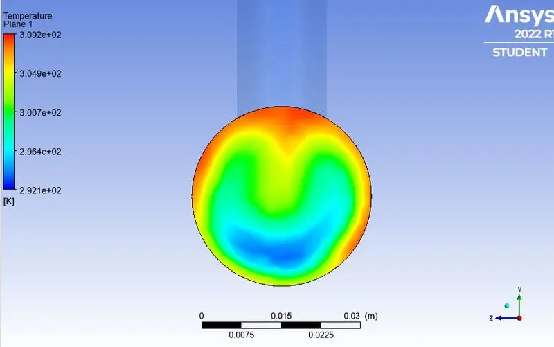
Fig. Temperature plot across the length of the pipe

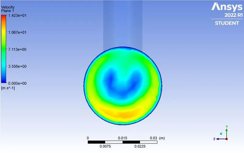
Fig. Velocity plot across the length of the pipe

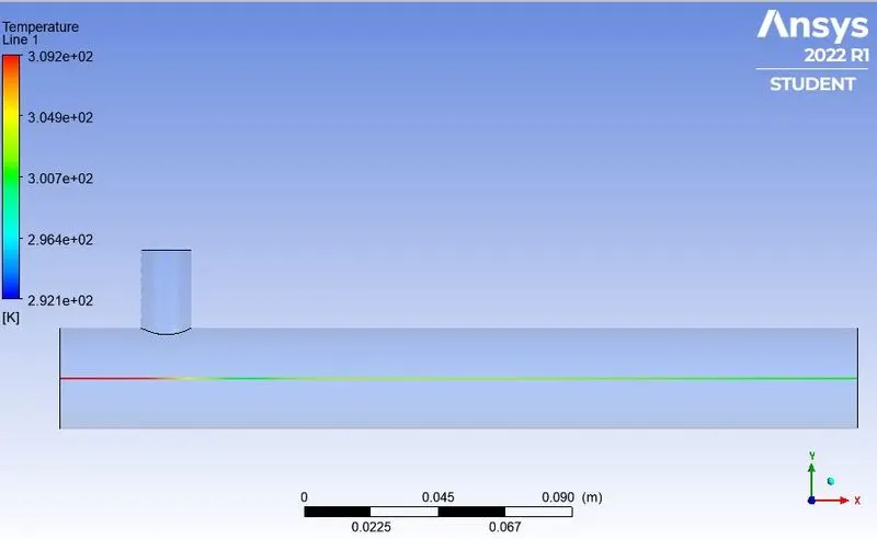
Fig. Temperature Line plot along the length of the pipe

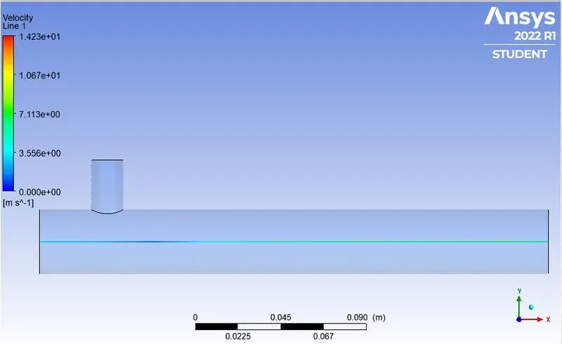
Fig. Velocity Line plot along the length of the pipe

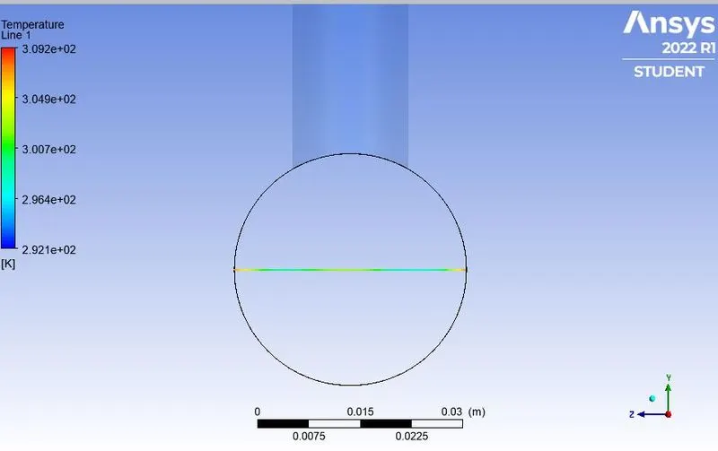
Fig. Temperature Line plot across the length of the pipe

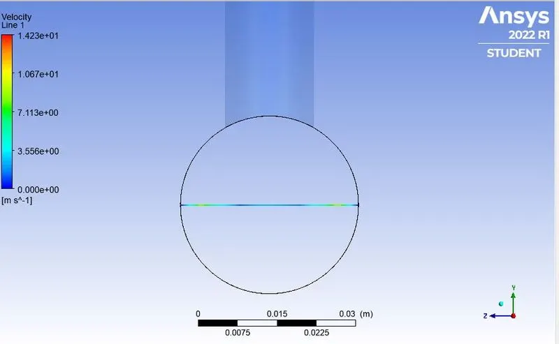
Fig. Velocity Line plot across the length of the pipe

# Plots and contours from k-omega model for short mixing tee @ momentum ratio = 4

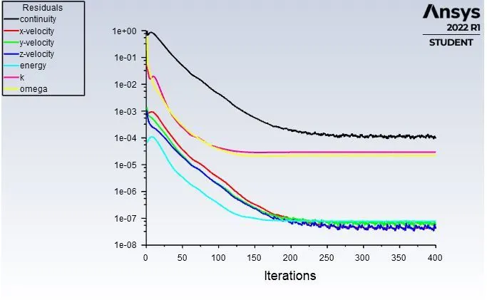
Fig. Residuals

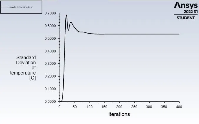
Fig. Standard Deviation of Temperature vs Iterations

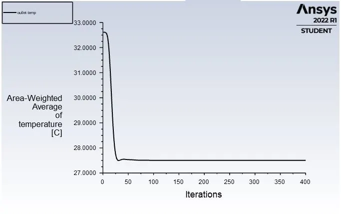
Fig. Average Temperature vs Iterations

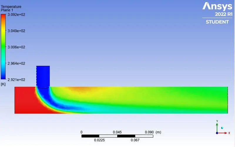
Fig. Temperature Contour along the length of the pipe

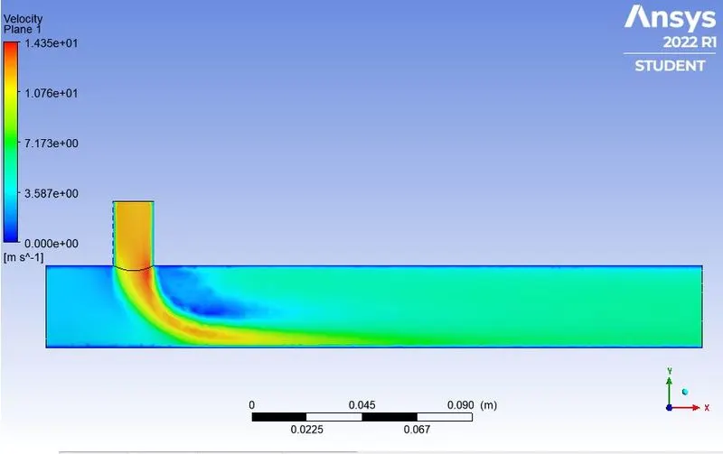
Fig. Velocity Contour along the length of the pipe

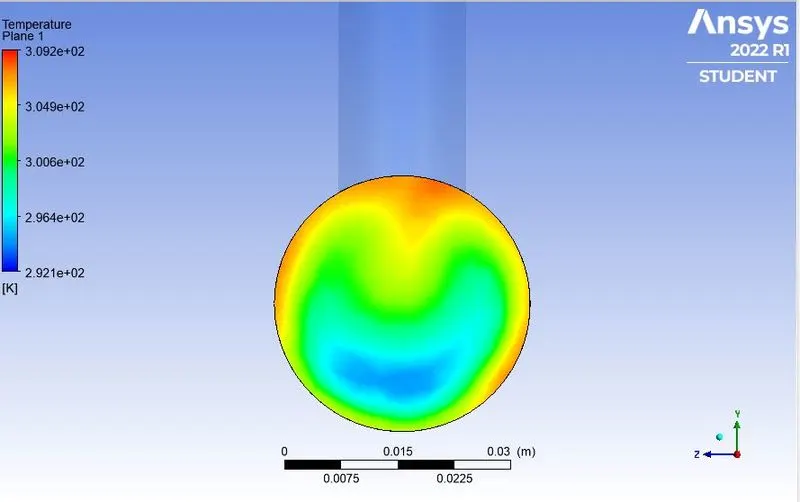
Fig. Temperature plot across the length of the pipe

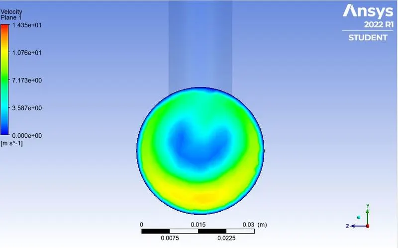
Fig. Velocity plot across the length of the pipe

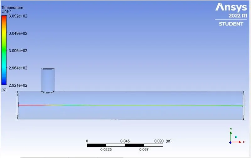
Fig. Temperature Line plot along the length of the pipe

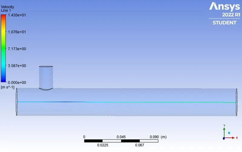
Fig. Velocity Line plot along the length of the pipe

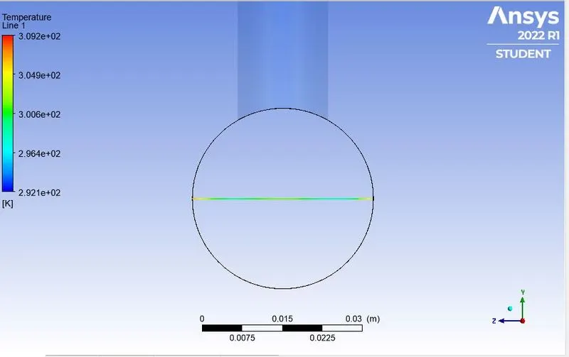
Fig. Temperature Line plot across the length of the pipe

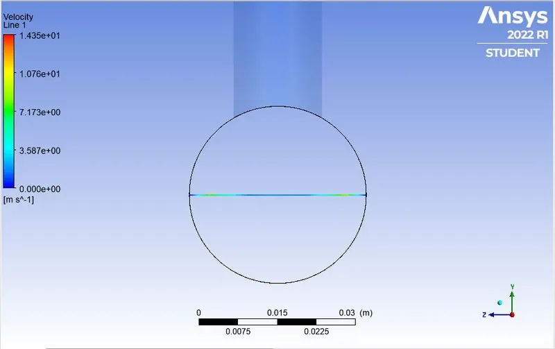
Fig. Velocity Line plot across the length of the pipe

Case 2 - In this case long mixing tee is used, which was mixing two fluid with temperature 36 & 19 degree C. Velocity of hot fluid was 3m/s and cold fluid was 12m/s.

we used realized k-epislon model and solution was converged after 180 iterations.

# Plots and contours from k-epsilon model for LONG mixing tee @ momentum ratio = 2

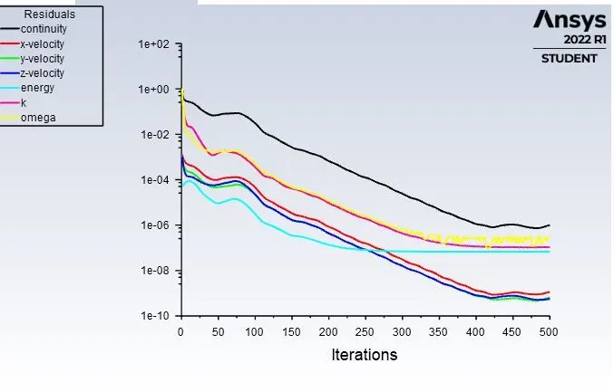
Fig. Residuals

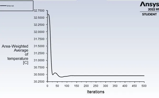
Fig. Average Temperature vs Iterations

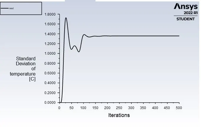
Fig. Standard Deviation of Temperature vs Iterations

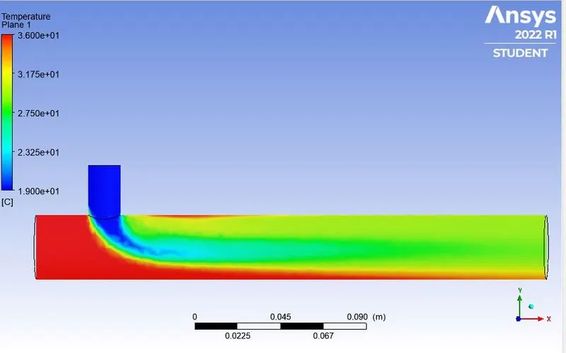
Fig. Temperature Contour along the length of the pipe

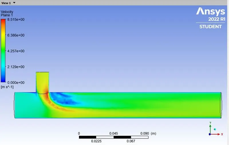
Fig. Velocity Contour along the length of the pipe

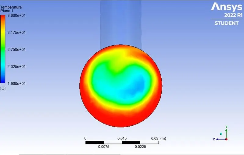
Fig. Temperature plot across the length of the pipe

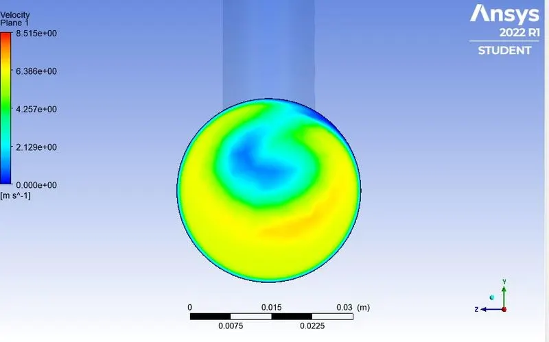
Fig. Temperature plot across the length of the pipe

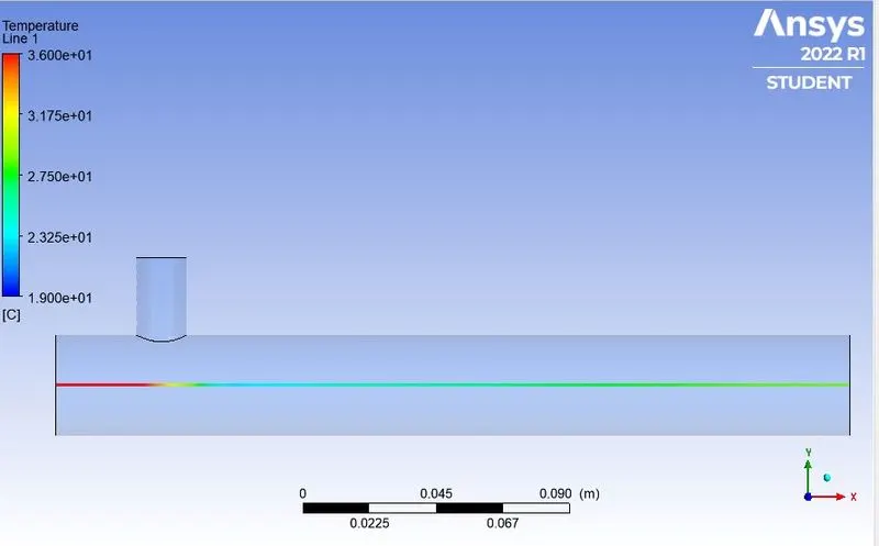
Fig. Temperature Line plot along the length of the pipe

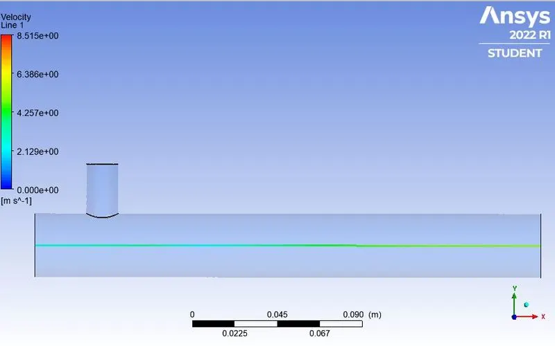
Fig. Velocity Line plot along the length of the pipe

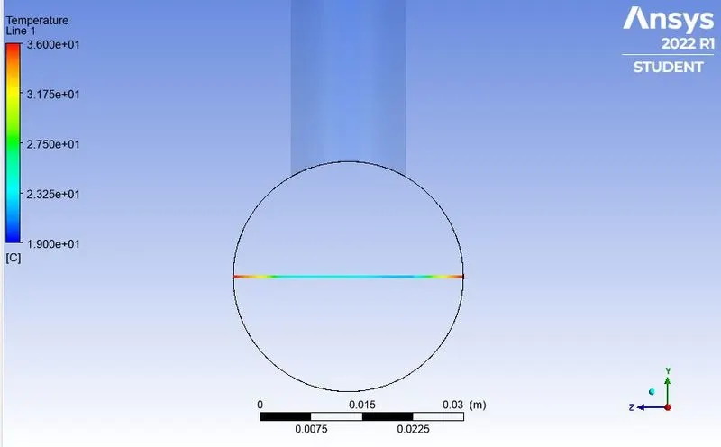
Fig. Temperature Line plot across the length of the pipe

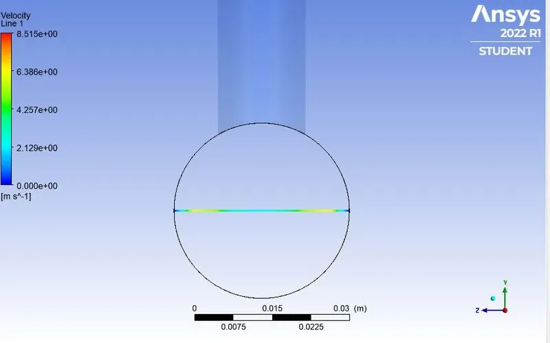
Fig. Velocity Line plot across the length of the pipe

# Plots and contours from k-epsilon model for LONG mixing tee @ momentum ratio = 4

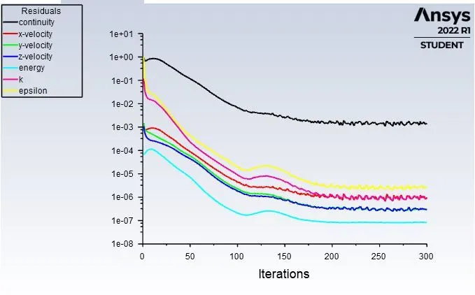
Fig. Residuals

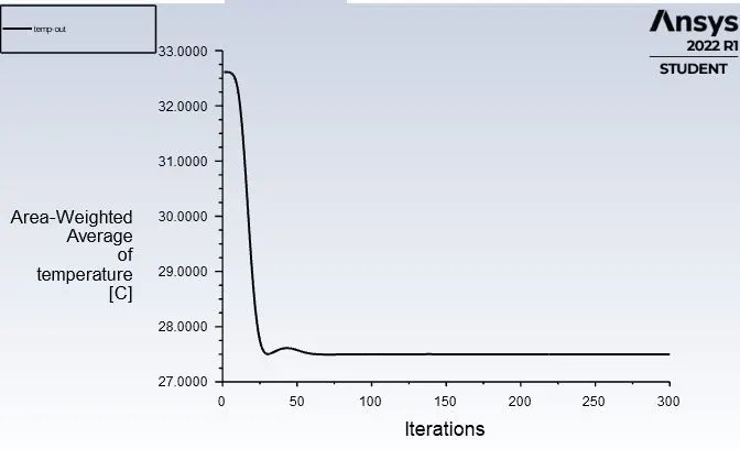
Fig. Average Temperature vs Iterations

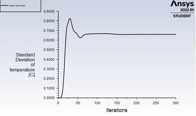
Fig. Standard Deviation of Temperature vs Iterations

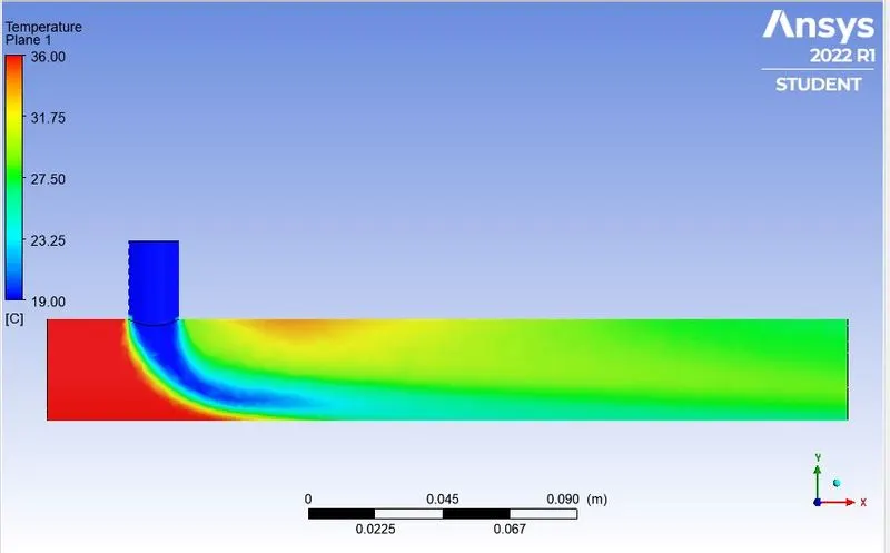
Fig. Temperature Contour along the length of the pipe

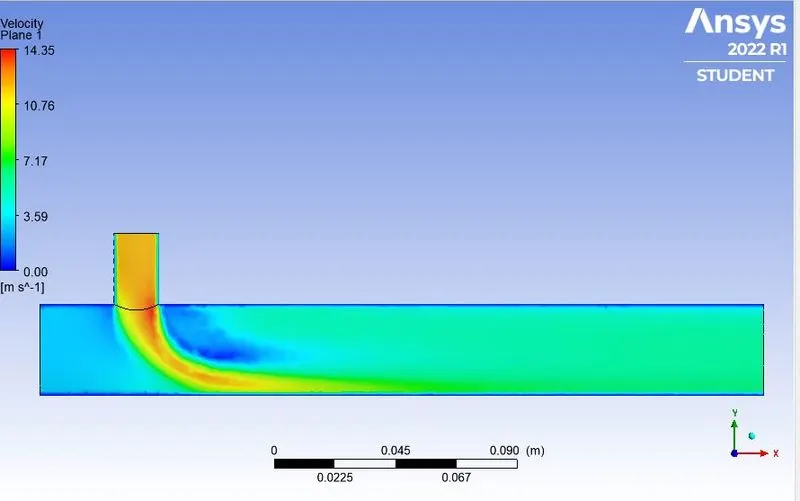
Fig. Velocity Contour along the length of the pipe

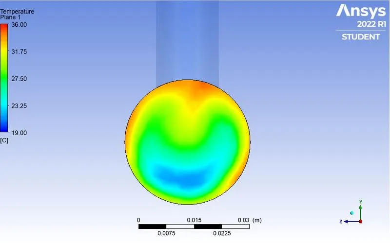
Fig. Temperature plot across the length of the pipe

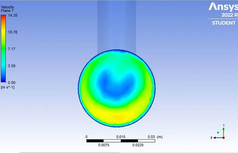
Fig. Velocity plot across the length of the pipe

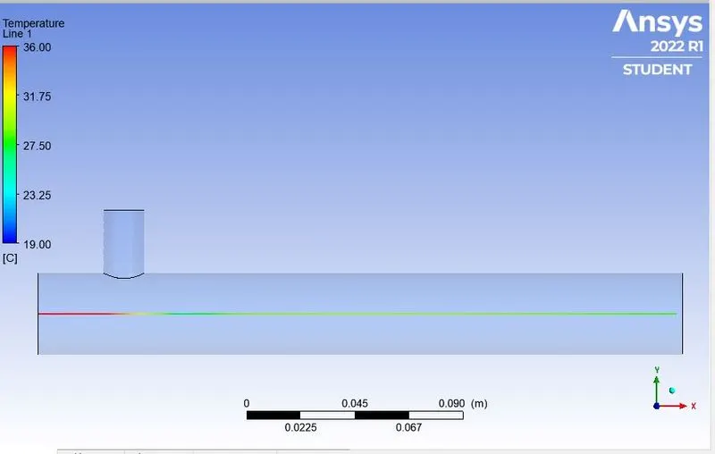
Fig. Temperature Line plot along the length of the pipe

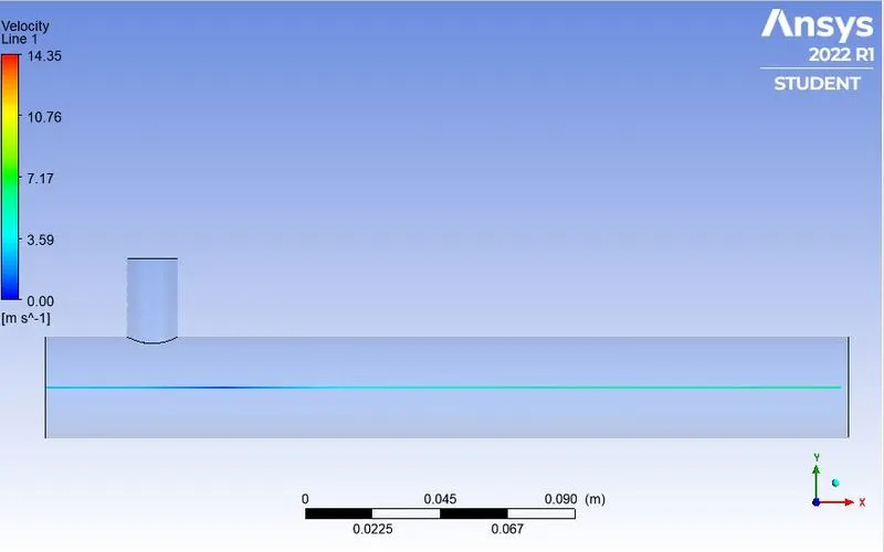
Fig. Velocity Line plot along the length of the pipe

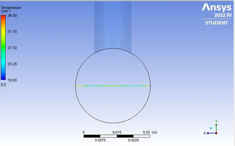
Fig. Temperature Line plot across the length of the pipe

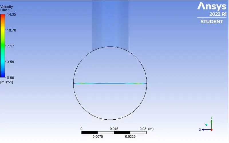
Fig. Velocity Line plot across the length of the pipe

LONG TEE

SHORT TEE

Parameters	Momentum Ratio = 2 k- Epsilon	Momentum Ratio = 4 k -Epsilon	Momentum Ratio = 4 k -Epsilon	Momentum Ratio = 4 k - omega	Momentum Ratio = 2 k -Epsilon	Momentum Ratio = 2 k - omega
Cell count/ No. of element	1,86,551	1,40,811	140811	140811	140811	140811
Standard Deviation	1.3557915	0.6591	0.659144	0.533	0.659144	0.53339
Outlet Temperature	30.4579	27.499	27.499	27.50	27.499	27.5033
No. of iteration at which solution converge	425	200	200	200	180	220

Analytical Approach -

Analytical formula for `T_mix` value at outlet is

`T_{mix} = [(m_{hot} * T_{hot}) + (m_{cold} * T_{cold})]/(m_{hot} +m_{cold})`

where m = mass flow rate

`T_{cold}` - Temperature at cold inlet = 19 degree C

`T_{hot}` - Temperature at hot inlet = 36 degree C

`T_{mix}`- outlet temperature after mixing

`A_{hot}` -= 901.3138 `mm^2` , `A_{cold}` = 225.9823 `mm^2` , `V_{hot}` = 3m/s , `V_{cold}` =12m/s

At Momentum ratio = 2 `T_{mix} = 30.3222`

At Momentum ratio = 4 `T_{mix} = 27.4876`

# By comparing both of the cases the analytical and numerical solution we can say that % of difference is very less

Effects of length and momentum ratioon results : -

• From above results we can say that outlet temperature is independent of length of the mixing tee.
• Momentum ratio effects the outlet temperature. By increases the momentum ratio outlet temperature is dropping.
• From above validation of numerical and analytical values we can say that numerical simulation values are matching with analytical values.

Mesh independent study : -

Here i took short mixing tee momentum ratio 2 cases.

Average Outlet No. of

MESH SIZE	No. of Element	No. of Nodes	Temperature (C)	No. of Iterations
5mm	18178	4020	27.49	200
4mm	28817	6196	27.51	190
3mm	56628	11724	27.54	175

Conclusion :-

• The mesh size of 3mm gives the best predicted results than other two mesh size.
• Decreasing the mesh size, the average outlet temperature starts approaching towards the analytical results
• A Short tee is preferred rather than Long Tee because short Tee has better mixing efficiency and low outlet temperature than long Tee.
• Hence, Momentum ratio 4 is more preferred over Momentum ratio 2 due to above- mentioned tables and reasons.
• Therefore, we recommended using the long tee and high-velocity inlet for application. This is because we have a
• The main advantage of this study is to decrease the computational time for solving.