Mixing Tee

Aim:

To compare the mixing effectiveness when a hot temperature and cold temperature fluid passed through a different Tees using K epsilon and SST omega Model and compare its values.

1. Case: 1
   • Short mixing tee with a hot inlet velocity of 3m/s.
   • Momentum ratio of 2, 4.
2. Case: 2
   • Long mixing tee with a hot inlet velocity of 3m/s.
   • Momentum ratio of 2, 4.

Given:

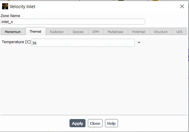
• Hot fluid inlet temperature = 36 degrees C
• Cold fluid inlet temperature = 19 degrees C

Introduction:

In CFD, the codes work through three processes:

• Pre-Processing.
• Solving.
• Post- Processing.

Pre-Processor:

• It consists of the Input of a flow problem.
• Definition of a geometry- Computational domain.
• Grid generation
• Selection of the physical and chemical phenomena.
• Definition of fluid properties.
• specification of appropriate boundary conditions at cells that coincide with or touch the domain boundary.

The solution to a flow problem is defined at nodes inside each cell. The accuracy of a CFD solution is governed by the number of cells in the grid.

Solver:

• Finite difference method
• Finite element method
• Spectral methods
• Finite Volume method

Post-Processor:

• Domain geometry and grid display
• Vector plots
• Line and shaded contour plots
• 2D and 3D surface plots
• particle tracking
• View manipulation
• Colour postscript output

Pre-Processing:

Import CAD model into Ansys:

• Open Ansys Workbench.
• 
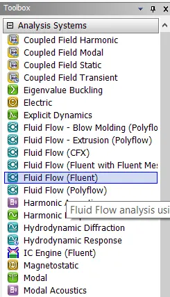
• Drag fluid flow (Fluent) from the toolbox to the Project schematic.
• 
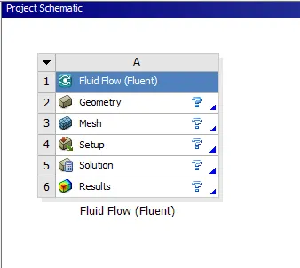
• Click on geometry to open the Ansys Space claim.
• Open File ⇒ New ⇒ Open the CAD file to perform stimulation.

Topological cleanup:

In the CAD model, we have both Solid and Fluid volume. We need fluid volume only to perform stimulation.

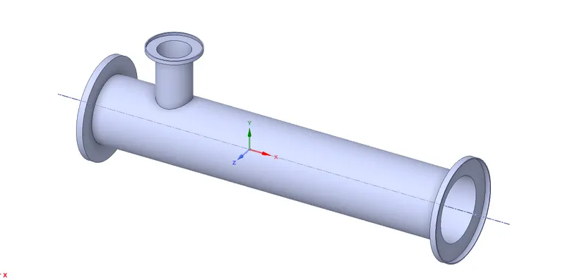
• Extraction of Fluid Volume:

Prepare option ⇒ Volume extraction ⇒ Edges Method⇒ Select appropriate edges and click Ok.

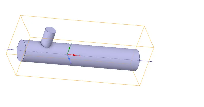
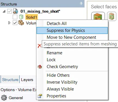
• To discontinue the solid volume from the Model, Use Suppress for the physics option. It helps to eliminate solid volume to proceed to further calculation.

Meshing:

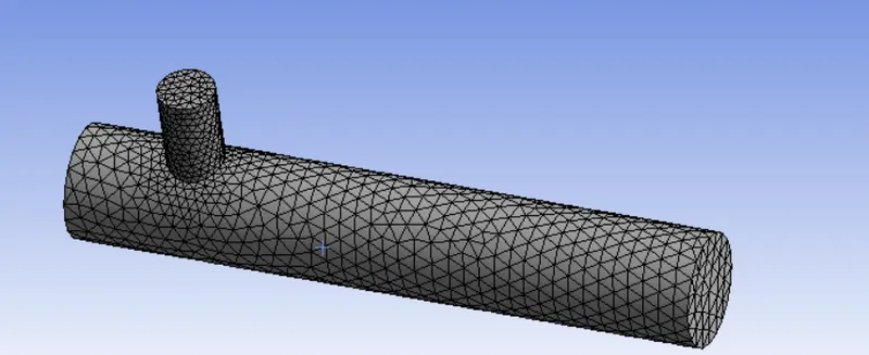
• After geometry, Click the Mesh option to create a mesh in the CAD Model.

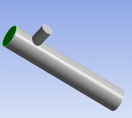
• Assigning Names to CAD Model, which helps to assign different properties at different entities in CAD Model easily.

1) Assigning inlet x ie. point of entry of Hot fluid:

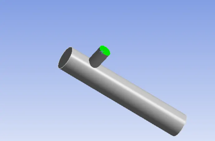
2) Assigning inlet y ie. entry point of cold fluid:

3) Assigning outlet ie. where the average outlet temperature is calculated (Result):

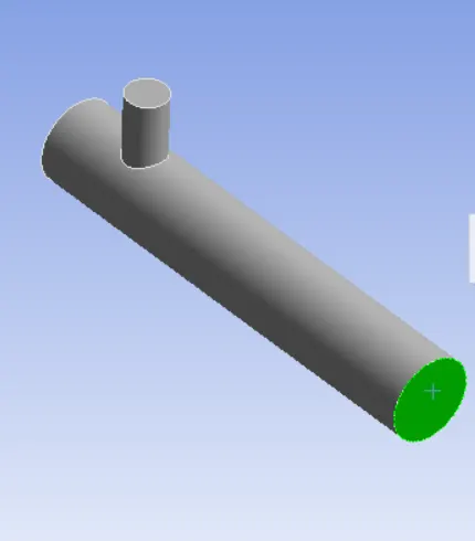
4) Assigning Walls ie. where the flow or stimulation takes place:

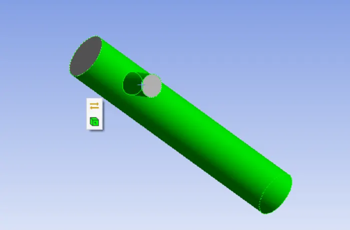
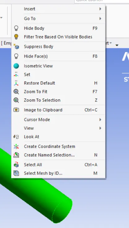
Above names can be assigned by click the right mouse button, create a named selection, or by using the shortcut button "N".

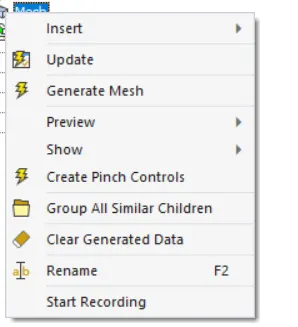
• Click Mesh option ⇒ Generate Mesh

Solver:

After topological cleanup and grid generation, the next step is to set solver. In solver, we are going to set up the physics required for stimulation.

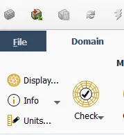
• In the First step, before assigning physics, we have to check the quality of the mesh.

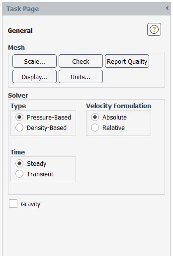
• Setting up the solver, for lesser mach no. we are going to use Pressure based steady solver with absolute velocity.

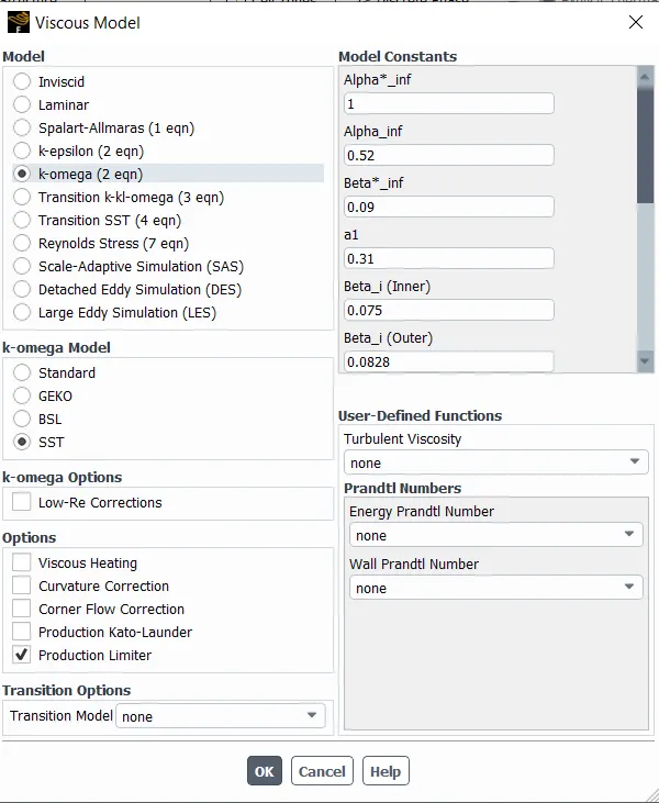
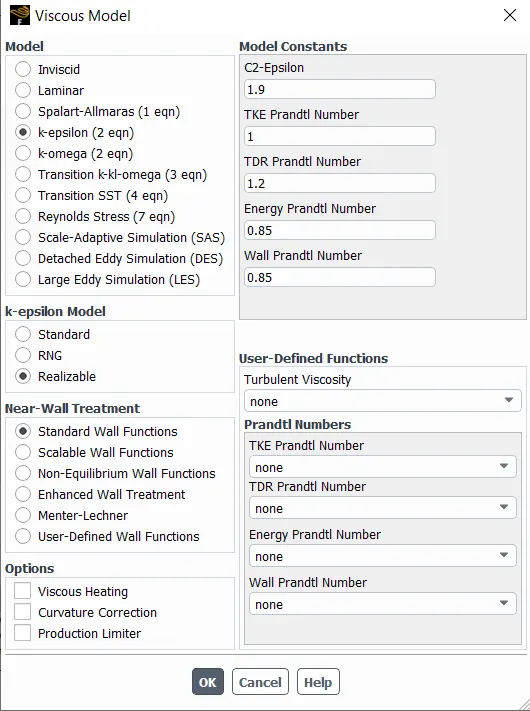
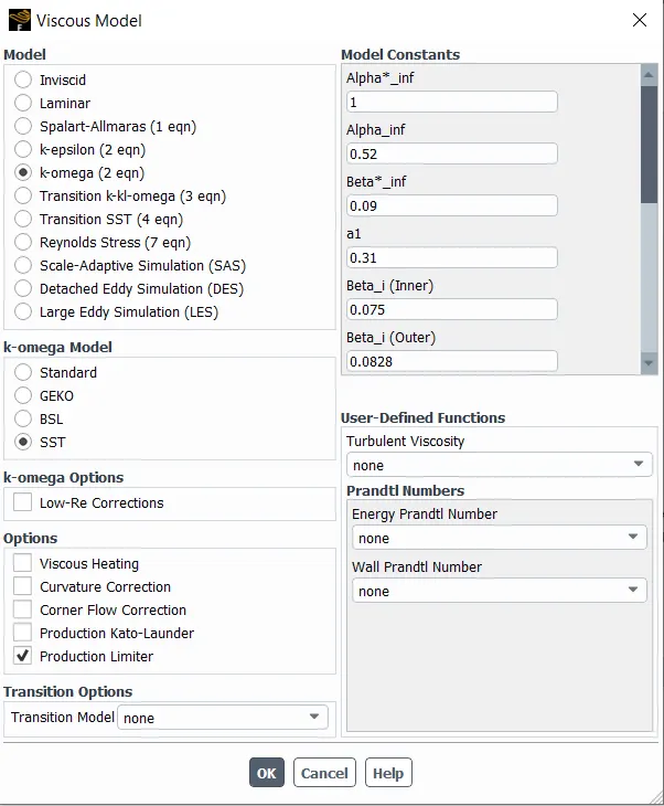
• Selecting Viscous Model

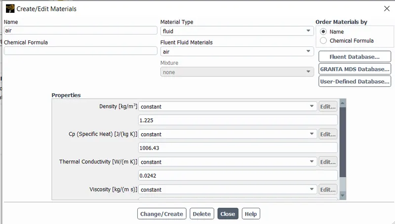
• The working medium in the stimulation is Air. It can be set up in Material Option.

• Assigning cell zones and Boundary conditions,

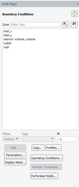
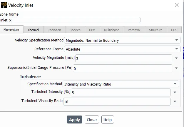
• Various conditions are assigned at different locations. After assigning boundary conditions step is to compute.
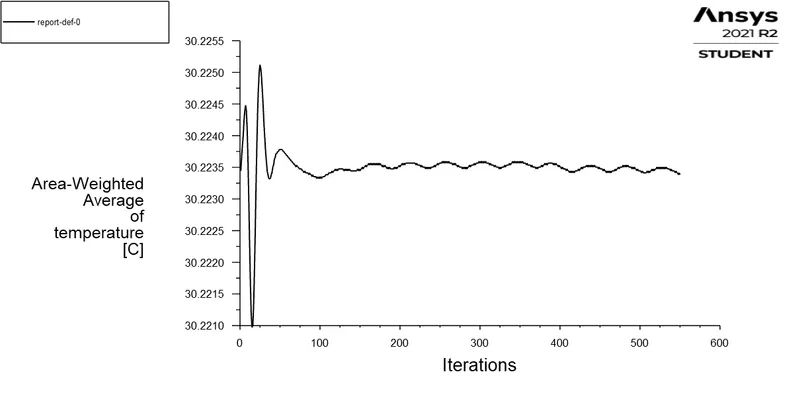
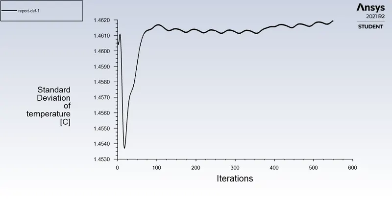
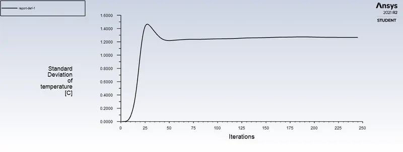
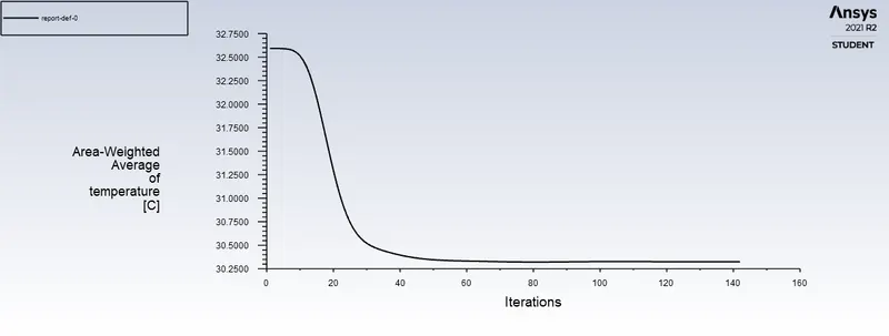
• Required Output plots are can be obtained from solutions ⇒ Definitions ⇒ Area weighted average and Standard deviation for Temperature at the outlet.
• Solution ⇒ Method(hybrid)⇒ initialize ⇒ Enter no. of iteration ⇒ Calculate.

Post-Processing:

• After solving the given problem, the results should be made easier to interpret the solution.

1. Case: 1
   • Short mixing tee with a hot inlet velocity of 3m/s.
   • Momentum ratio of 2, 4.

K- Epsilon:

Short mixing tee of Momentum ratio = 2:

• Hot inlet velocity of 3 m/s and Hot inlet temperature 36 degrees celsius.
• Cold inlet velocity of 6 m/s and Hot inlet temperature 19 degrees celsius.

Plots:

Temperature Contour plot:

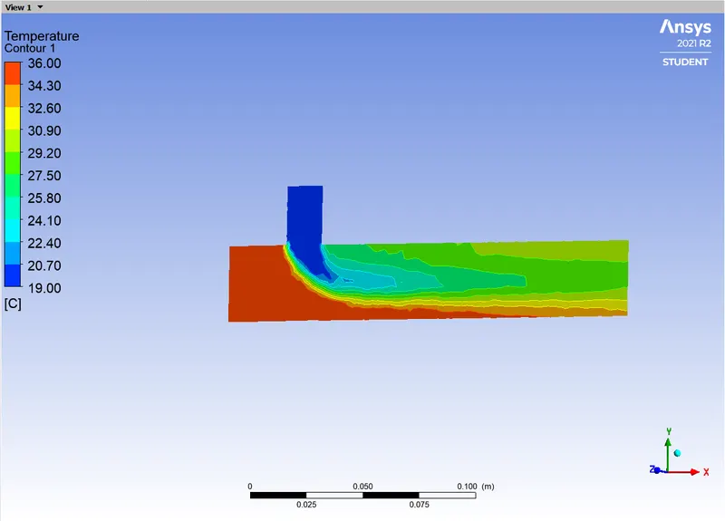
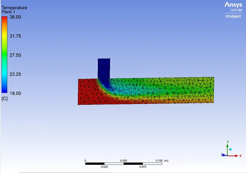
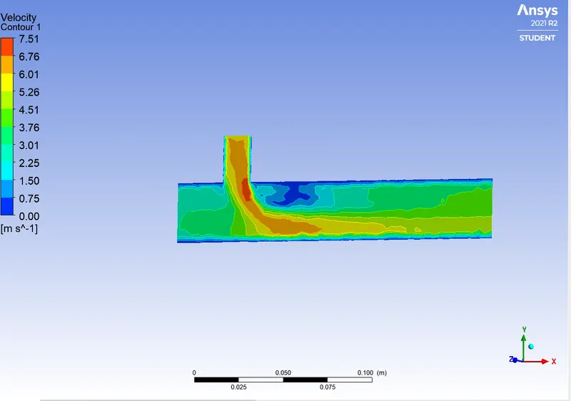
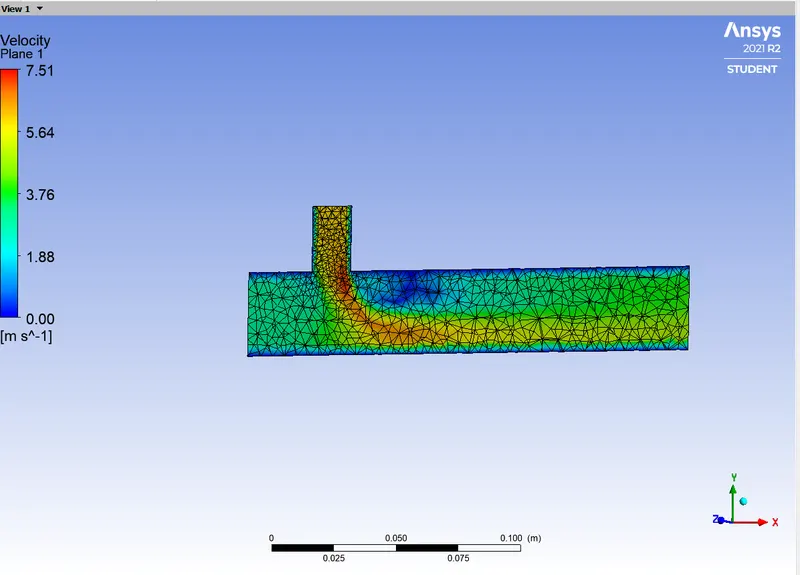
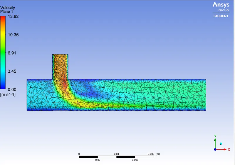
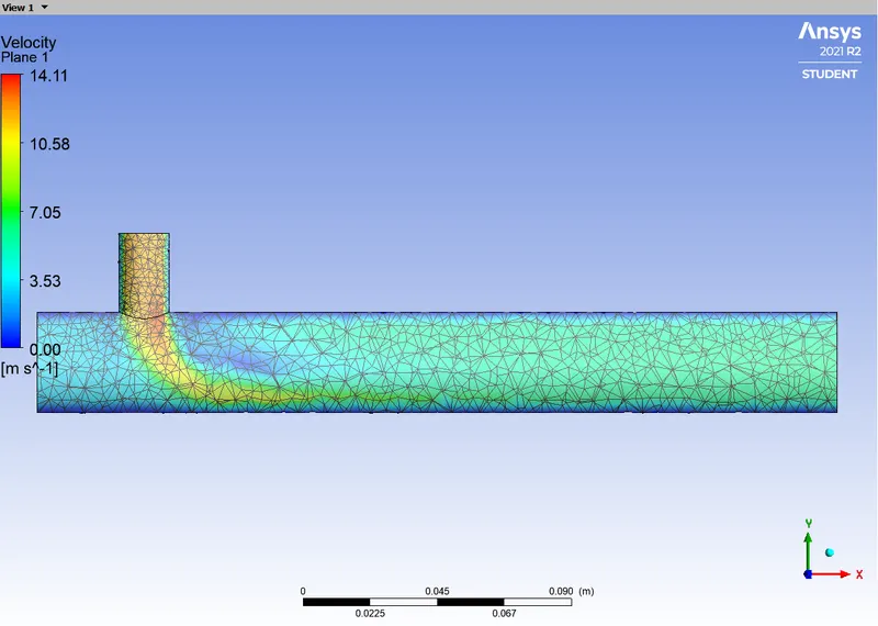
Velocity contour plot:

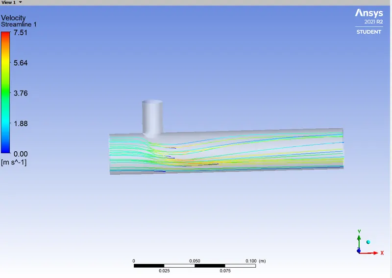
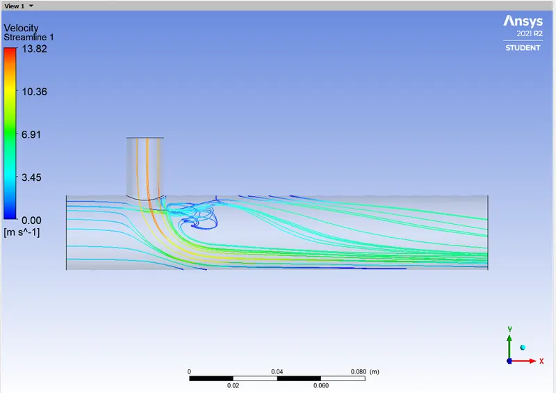
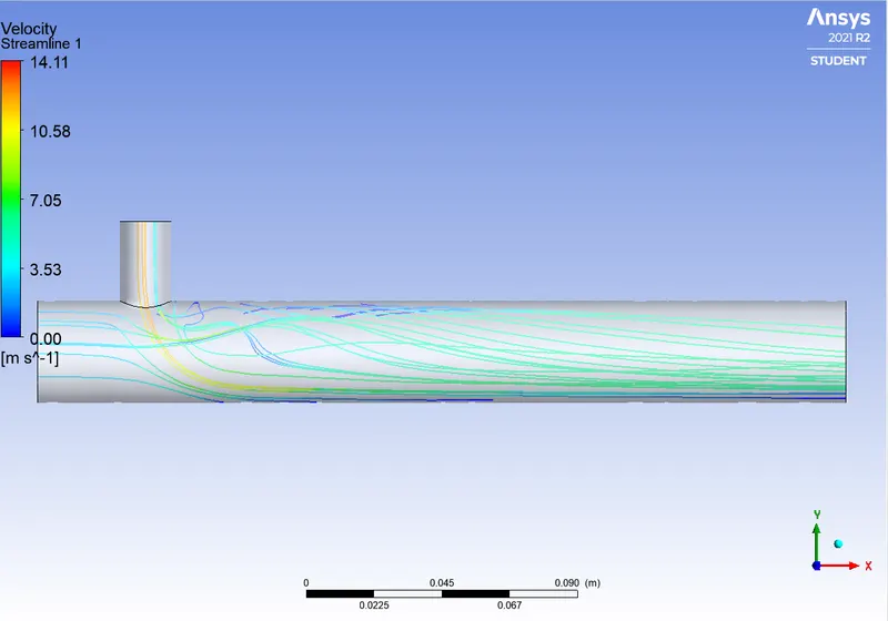
Velocity steam line plot:

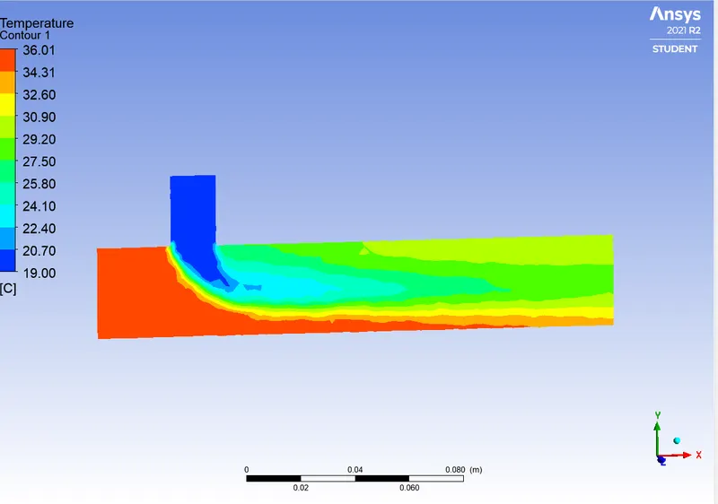
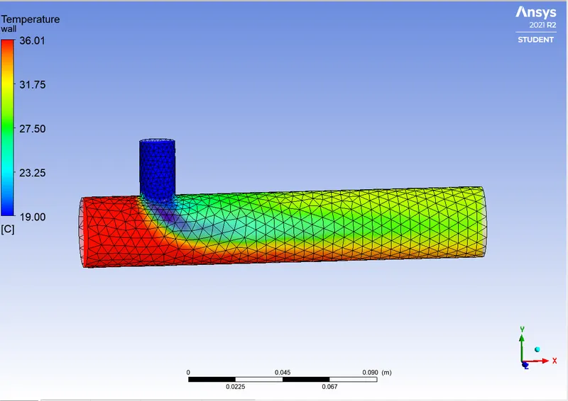
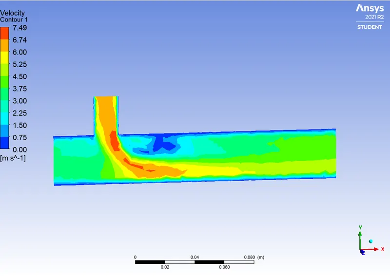
Omega SST Model:

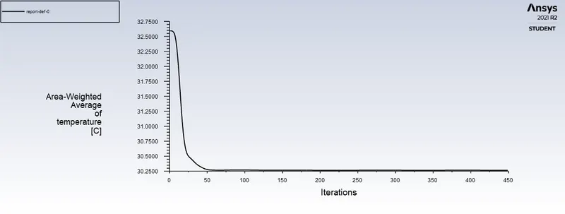
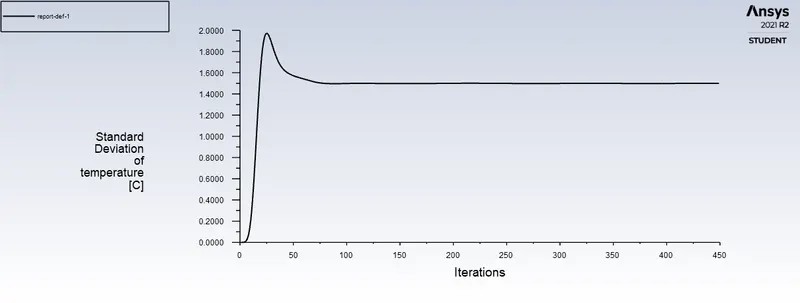
Temperature plot:

Velocity plots:

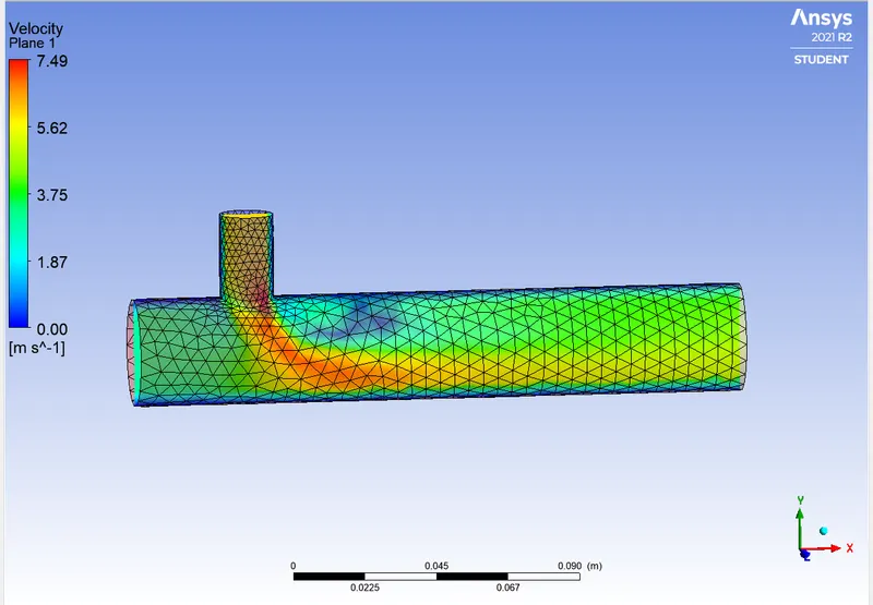
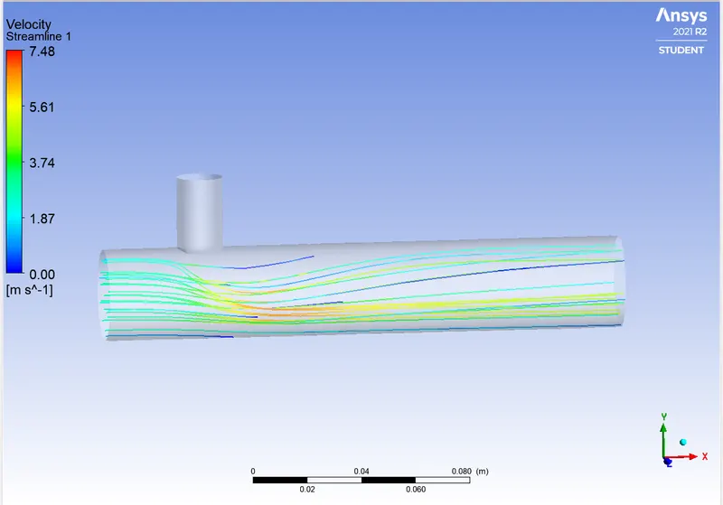
Comparing Mixing effectiveness using K-Epsilon and Omega SST models, When Hot inlet of Temperature 36 degrees celsius and Cold inlet of temperature 19-degree Celsius is passed through different ports of Tee.

Analytical calculation:

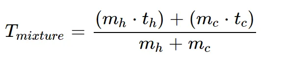
Where mh and mc is the mass flow rate of hot and cold inlet resp.

th and tc is the temperature of hot and cold inlet resp.

m_h = 1.225*0.0009*3;

m_h = 0.00330 kg/sec.

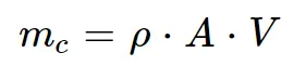
m_c = 1.225 *0.0002*6;

m_c = 0.00147 kg/sec.

t_h = 36;

t_c = 19:

substituting m_h,m_c, t_h and t_c in the above equation:

therefore,

T_Mixture = ((0.0033*36)+(0.00147*19))/(0.0033+0.00147);

T_mixture = 30.761 degree celsius.

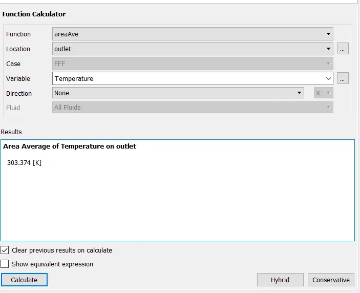
K- Epsilon Model:

T_mixture = 303.374 [K]

T_mixture = 30.224 C

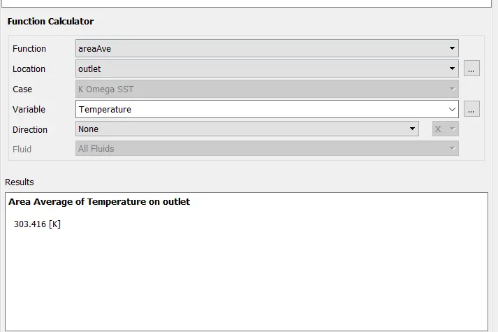
Omega SST model:

T_mixture = 303.416 K

T_mixture = 30.266 C

In order to find the most suitable model we have to compare with analytical vs stimulated results:

Error_Epsilon = T_mixture_analytical - T_mixture_epsilon model

Error_Epsilon = 30.761 - 30.224

Error_Epsilon = 0.537

Error_Omega = T_mixture_analytical - T_mixture_Omega Model

Error_Omega = 30.761 - 30.226

Error_Omega = 0.535

From the above result, we can say that the Omega SST model has a lesser error when compared to the K Epsilon model.

Omega SST model is used in future calculations.

Short mixing tee of Momentum ratio = 4:

• Hot inlet velocity of 3 m/s and Hot inlet temperature 36 degrees celsius.
• Cold inlet velocity of 12 m/s and Hot inlet temperature 19 degrees celsius.

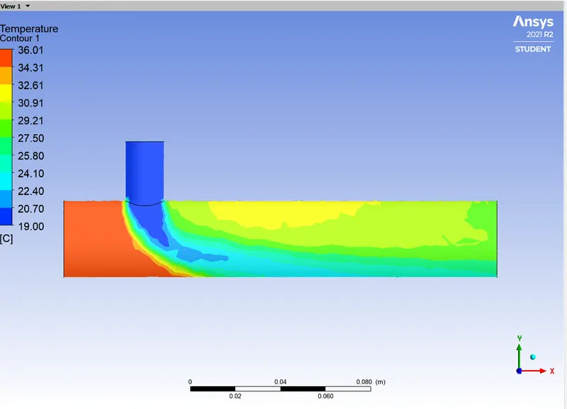
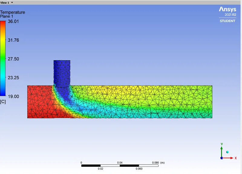
Temperature plots:

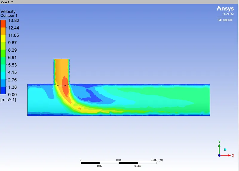
Velocity plots:

Case: 2

• Long mixing tee with a hot inlet velocity of 3m/s.
• Momentum ratio of 2, 4.

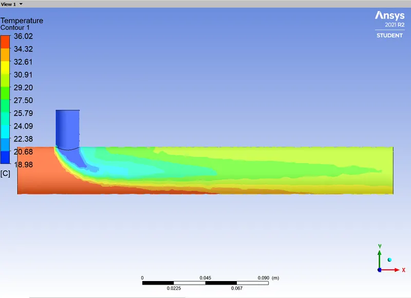
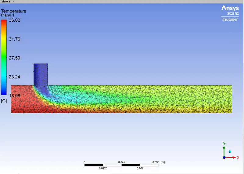
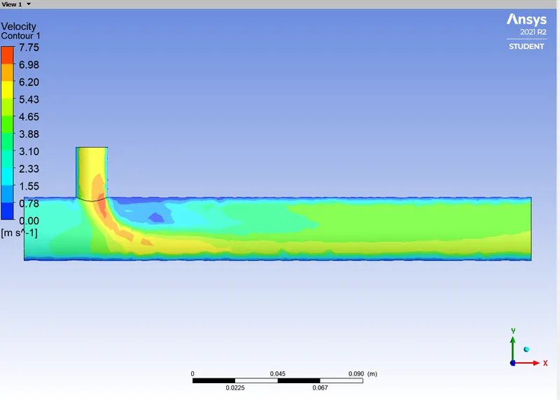
Long tee with Momentum ratio of 2:

Temperature plots:

velocity plots:

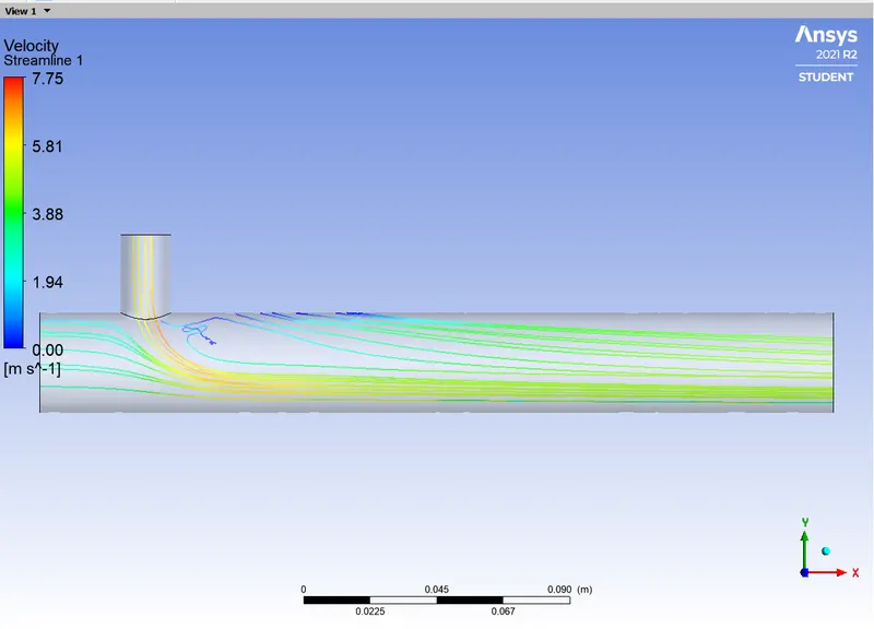
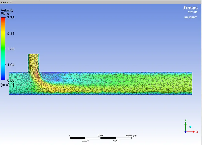
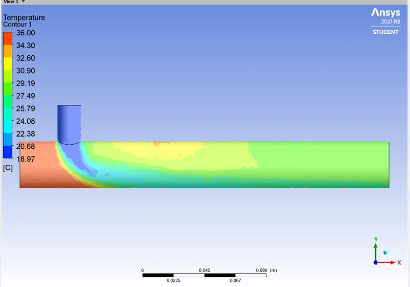
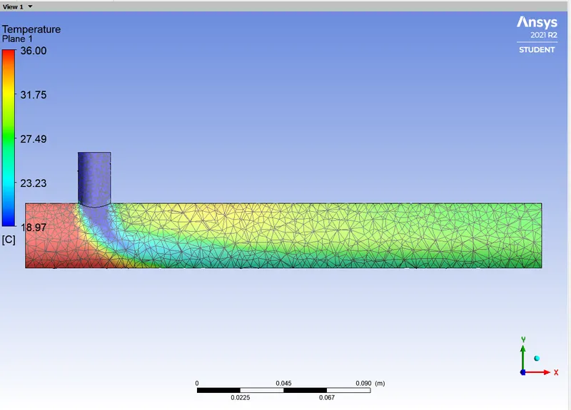
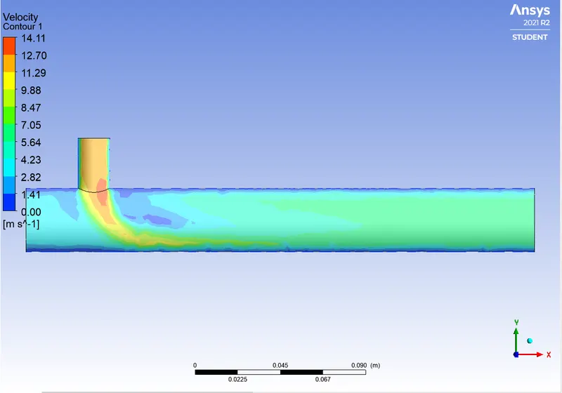
Long Mixing Tee with Momentum ratio of 12 m/s:

Temperature plots:

Velocity plots:

Tabulation:

S.No	Case	Cold Inlet velocity [m/s]	Number of elements	Outlet temperature[K]
1	1	6	12632	303.415
2		12	12632	300.68
3	2	6	15343	303.475
4		12	15343	300.641

Mesh/Grid Independent Test:

In Mesh independent test, the size of the mesh is varied. Due to variations in mesh we know that stimulation time increases.

No. of elements: 56003

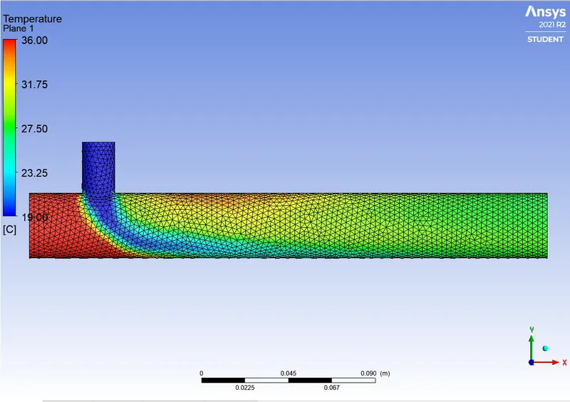
After:

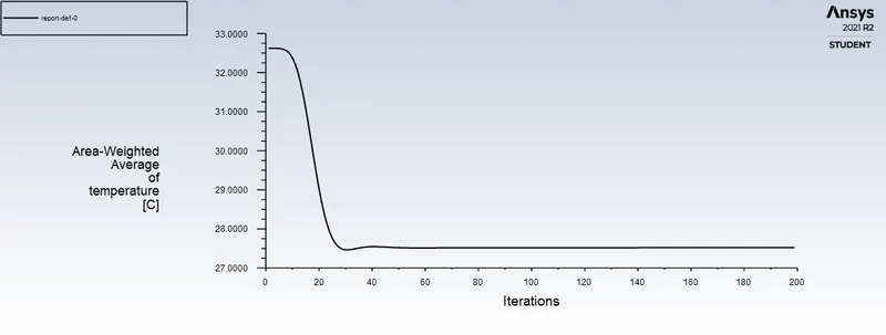
Before:

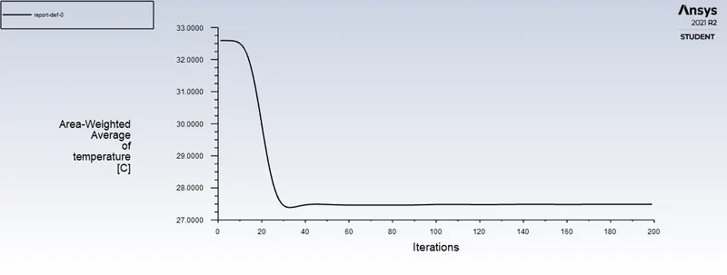
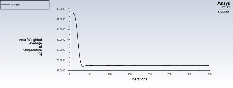
Outlet Temperature before refinement: 27.491 [C]

Outlet Temperature after refinement: 27.52 [C]

From the above the result, we came to know that the variation in mesh parameters does not affect the output results.

Result:

From the stimulated results,we can say that in the both the cases mixing effectiveness increases with increase in velocity so that the outlet temperature decreases as a result of efficient of mixing of cold inlet.

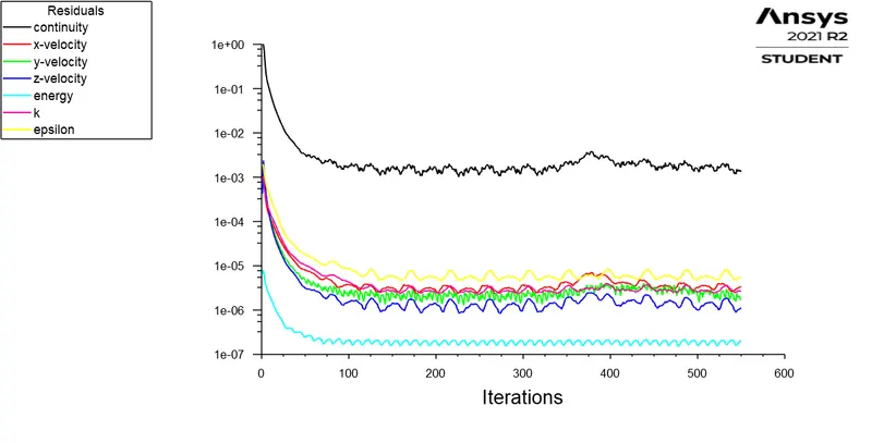
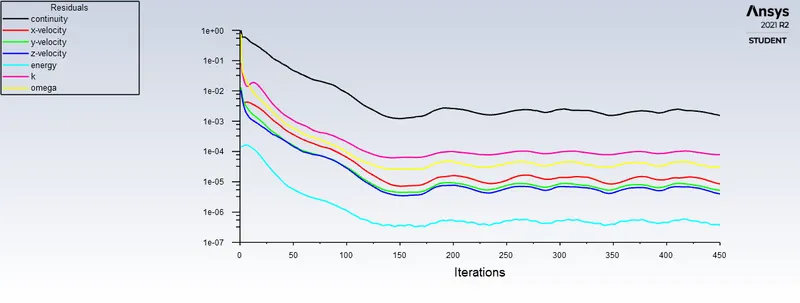
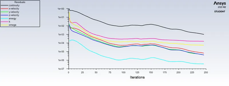
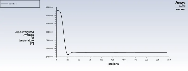
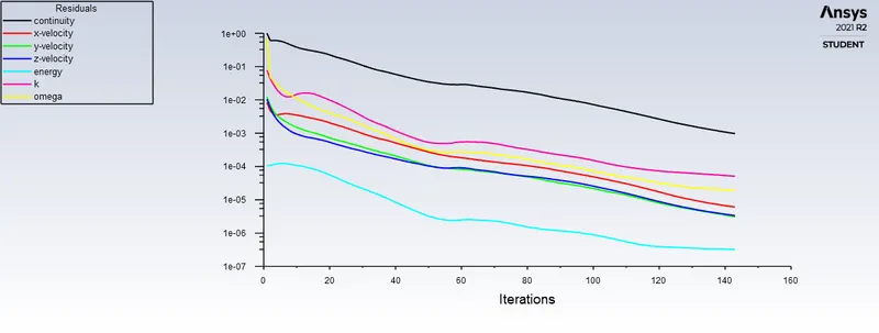
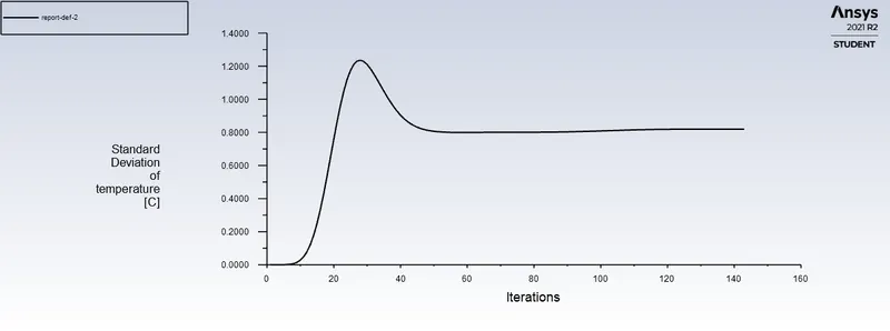
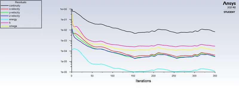
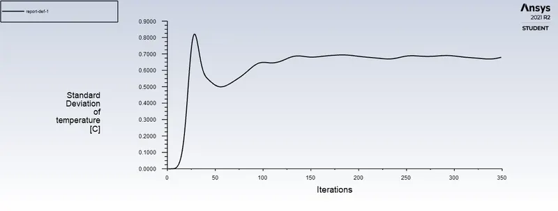
We can say that, if the plot tends to be steady/the pattern of the curve continuous the solution is said to be converged.