Week 1: Channel flow simulation using CONVERGE CFD

OBJECTIVE: TO SIMULATE A CHANNEL FLOW USING CONVERGE CFD

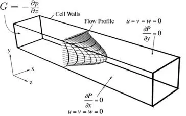
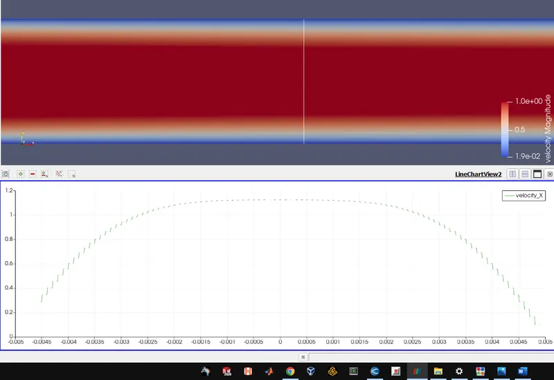
THEORY: The flow through a rectangular channels attains a parabolic profile due to the 0 velocity near walls because of No slip condition and when we move vertically towards the centre of the cross-section of rectangular channel we observe that the flow attains its maximum value of there which results in a parabolic profile of the floe/velocity.

PROCEDURE:

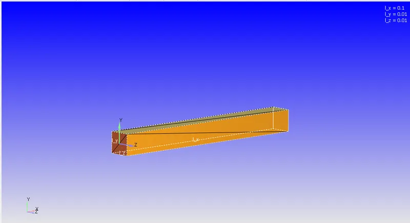
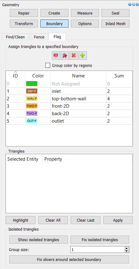
The rectangular channel of the dimensions (x=0.1 y=0.01 z=0.01) was created using 'create' tool after which we used the boundary tool to select the entities of boundaries and also assign them names accordingly.

After creating the channel and setting up the boundary we went to setup the case setup for which the case setup tree was generated by clicking on 'begin case setup' and then it was setup sequentially.

Application type was selected to be time-based simulation.

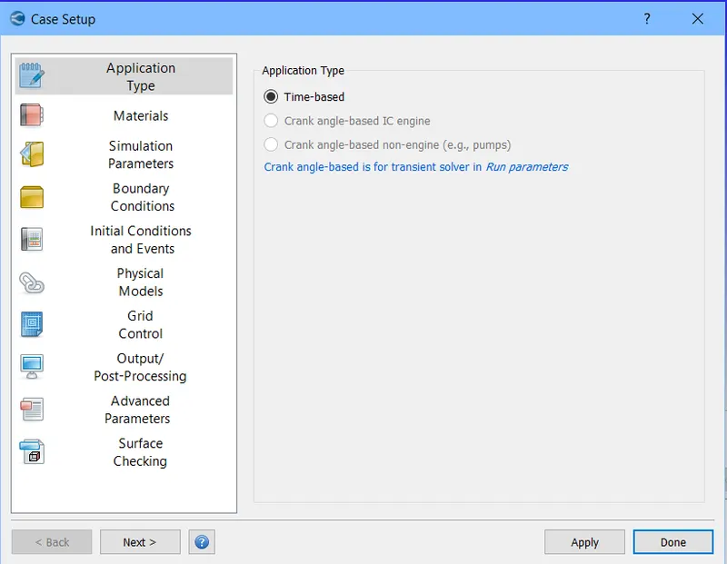
After selecting the application type materials were selected in which preddefined mixture was selected to be air species were enabled and reaction mechanism was dissabled.

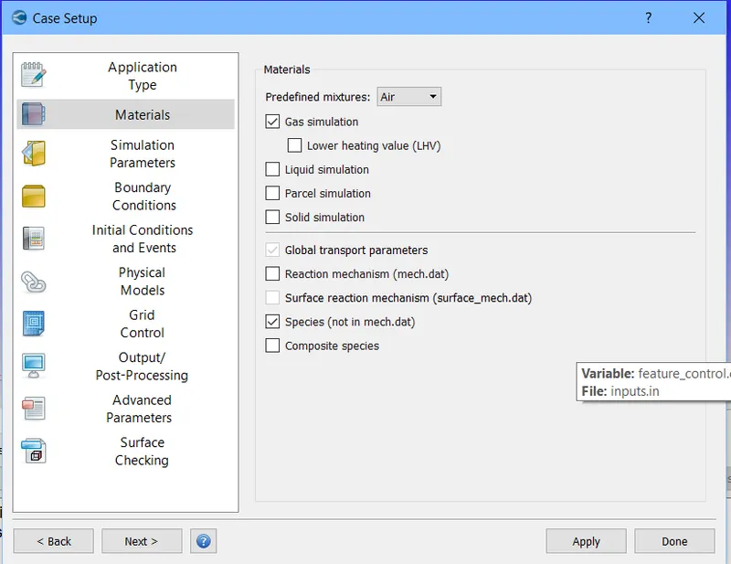
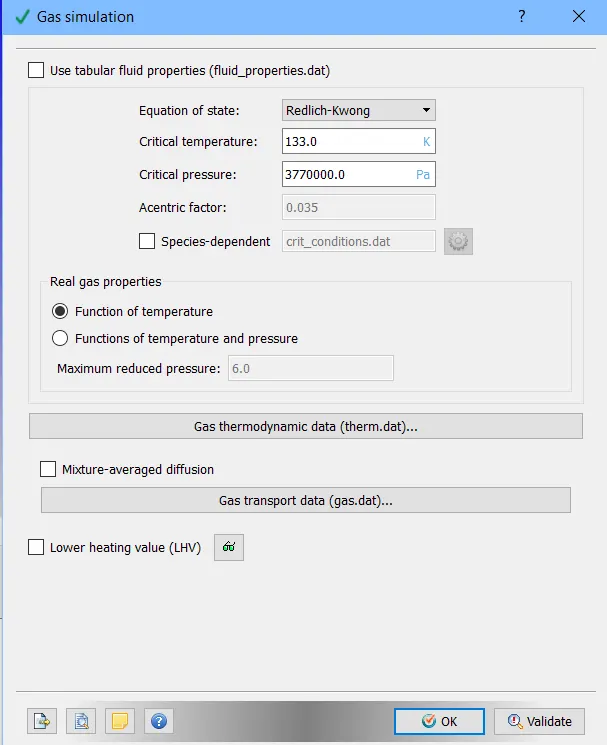
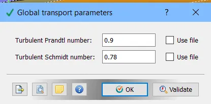
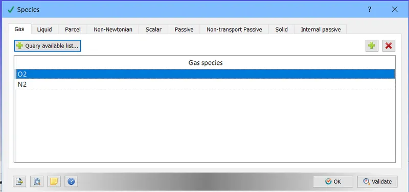
After this gas simulation parameters and global parameters was set to their default values and O2 and N2 were added into the species.

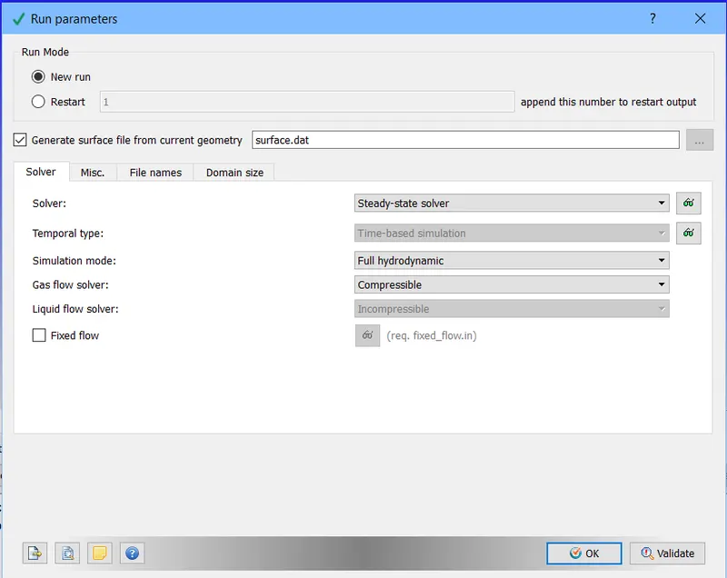
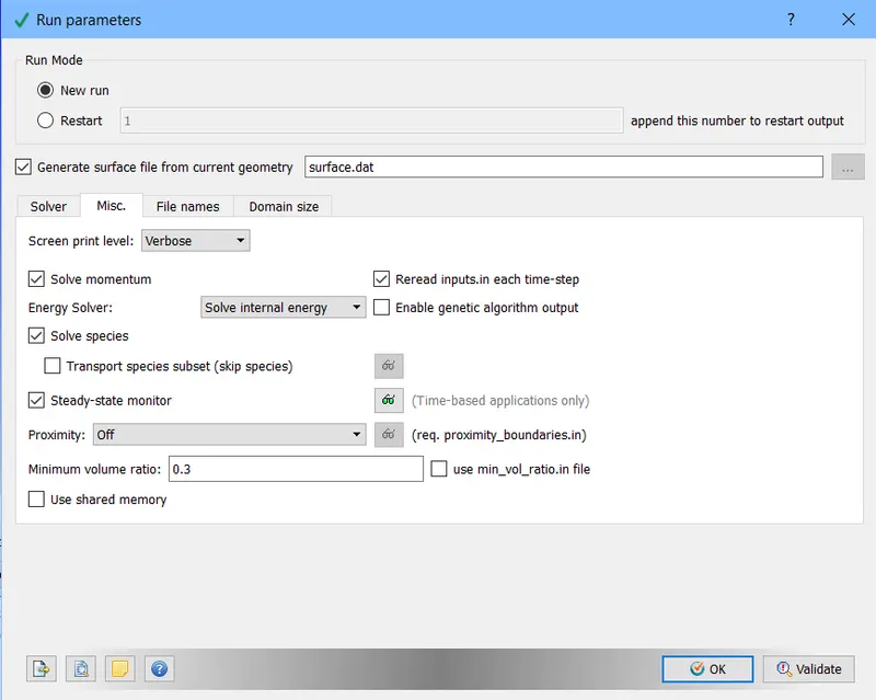
After this Run parameters were setup in which solver was selected to be steady-state solver and simulation type was hydradynamic simulation and gas flow solver was compressible and in the misc of the run parameters we unchecked share memory and steady-stae monitor was enabled.

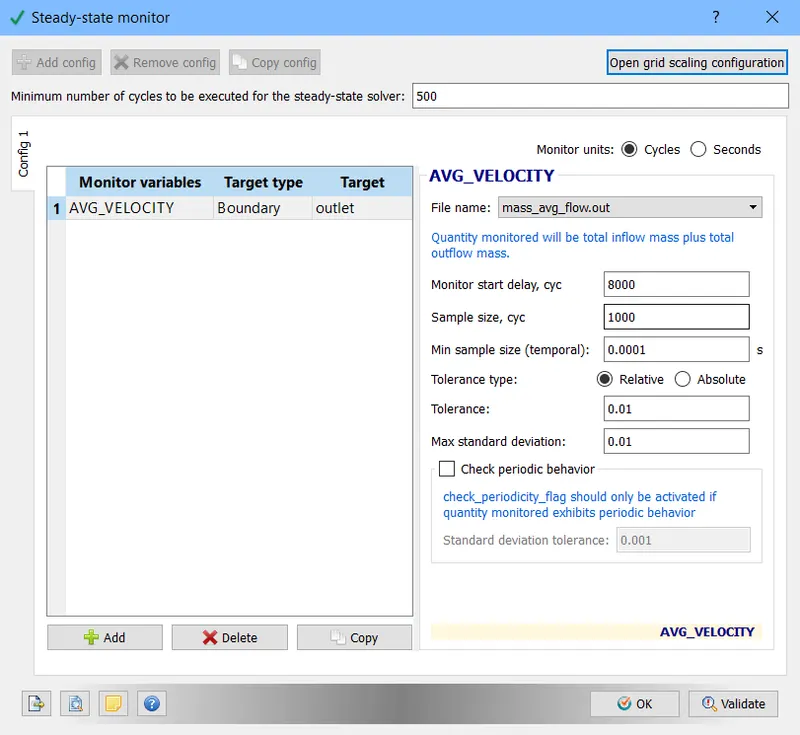
After this steady-state monitor was setup and the minimum number of cycles to be executed was set to 500 and monitor start delay was set to 8000 and sample size was set to 1000 cycles. with tolerance being 0.01 and the varuable to monitor was set to avg velocity at outlet.

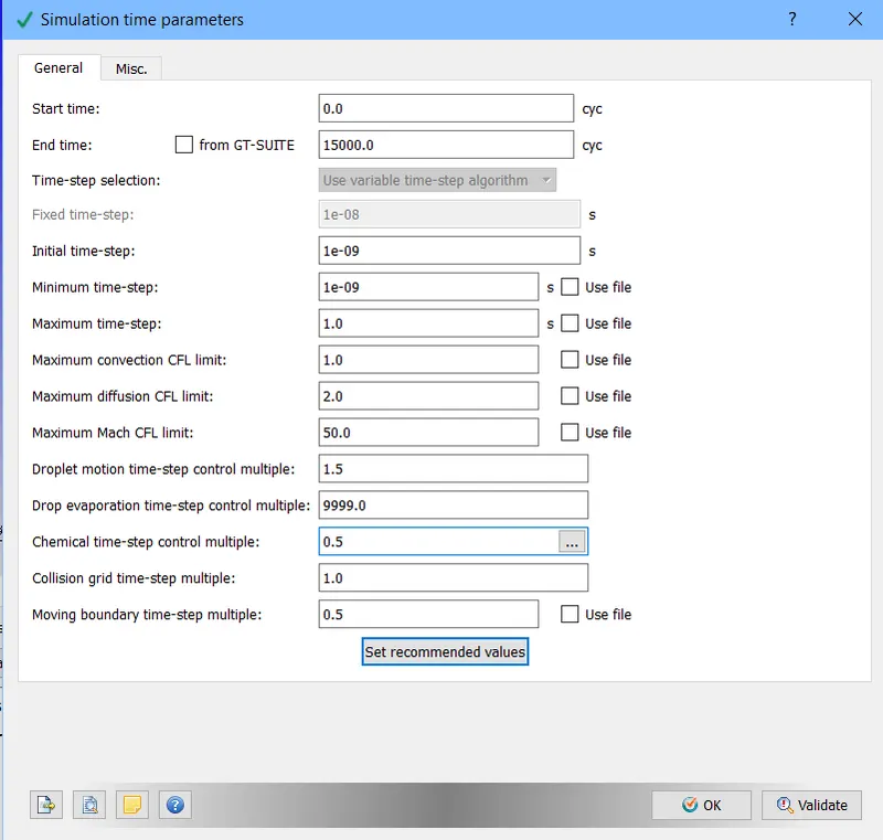
After this we went ahead and setup simulation time parameters where the start time was set to 0 and end cycle was selected to be 15000 and the initial and minimal time step was set at 1e-9 and maximum time step was set to 1. Rest settings were left at default values only.

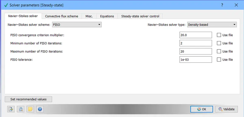
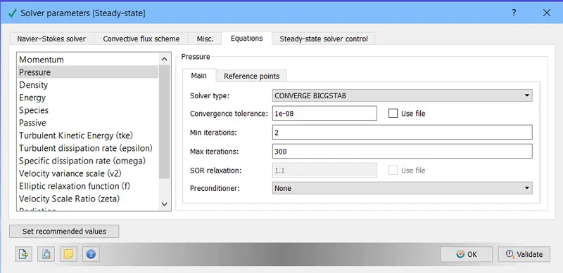
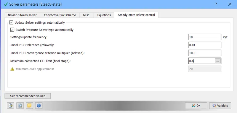
After this we setup solver parameters where the NS-solver scheme was set to PISO as it is fast and the NS-solver type was set to density-based solver and rest values were set to default and in the equations section we made sure that preconditioner for pressure is set to none. and maximum CFL in steady--state solver was set to a value below 1 here it was 0.8

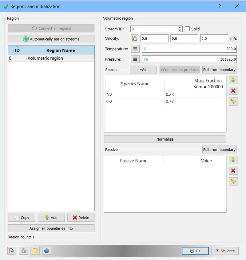
After this in region and initialisation we setup a region called volumteric region to which all the boundaries were assigned in the boundary setup. N2 and O2 was added to this region with their mole fraction or their composition being inversed i.e., O2 had 0.77 and N2 had 0.23 moles in 1 mole of air.

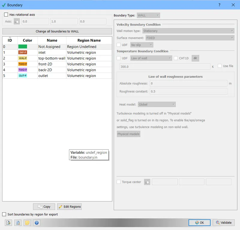
After this we went ahead to setup our mesh for which we used the values provided with the question.

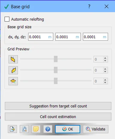
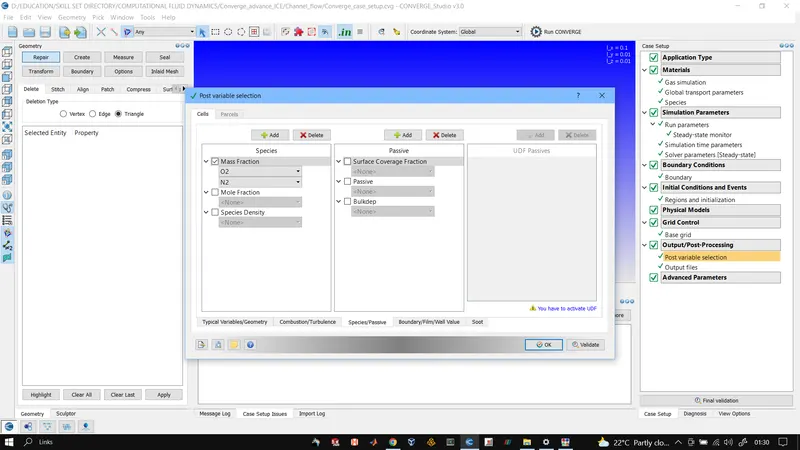
and after this post-variable setup was doen where all the turbulence setup were unchecked and required variables were selected in typical variable and O2 and N2 were added to species as mass-fractions.

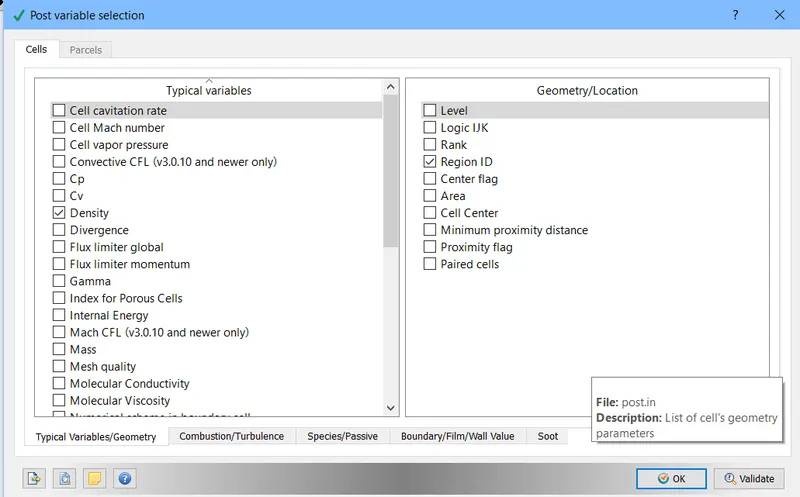
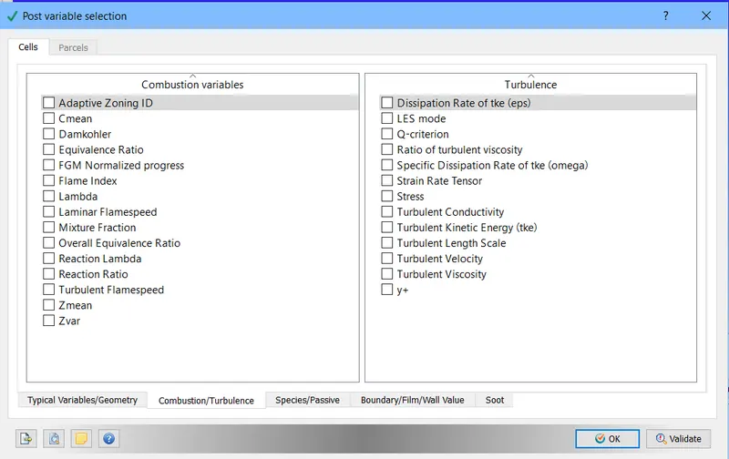
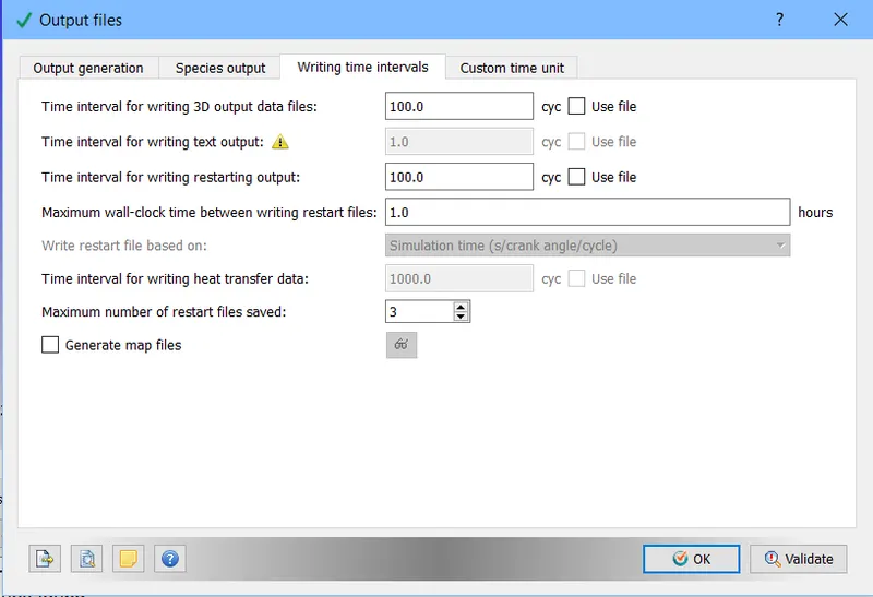
After this output files setup was completed where we setup the parameters for output file generation and number of restart files to generate and their time interva for generation.

After completing all are setups we validated to look for any error in the case setup.

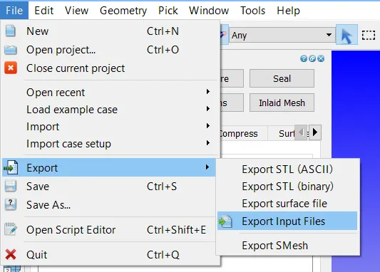
After getting a successful validation check we exported our input files into a folder which were later simulated using cygwin and then post converted to VTK binary format to post-process in paraview.

RESULTS:

CASE1 MESH SIZE 2e-4

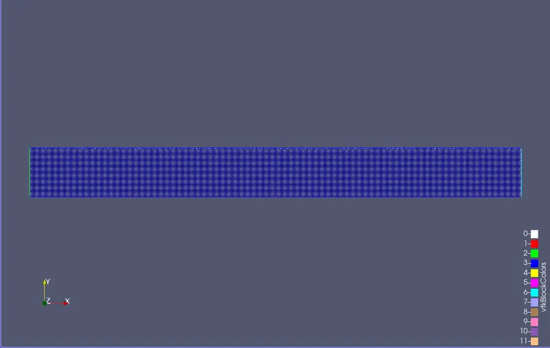
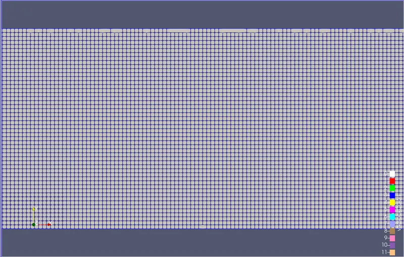
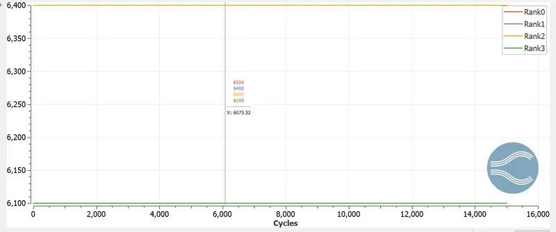
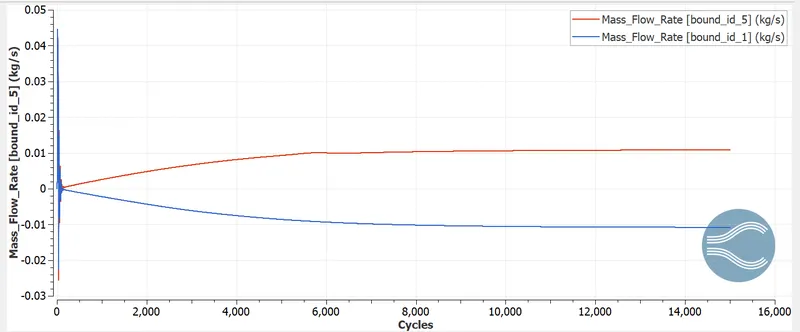
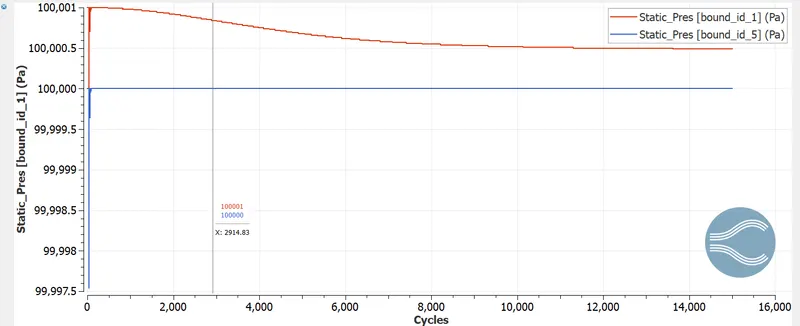
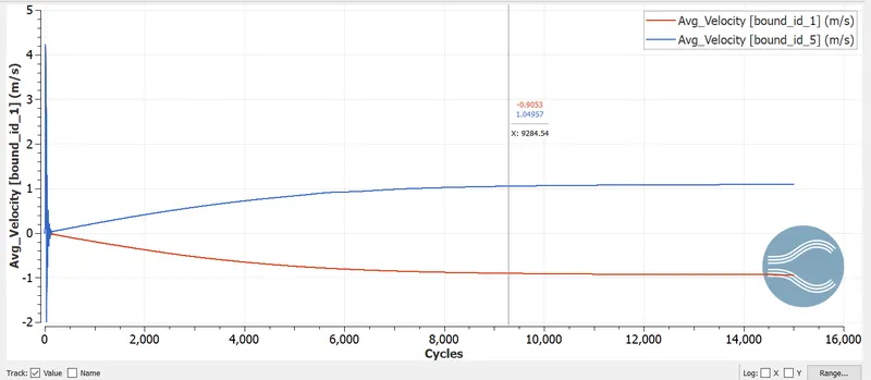
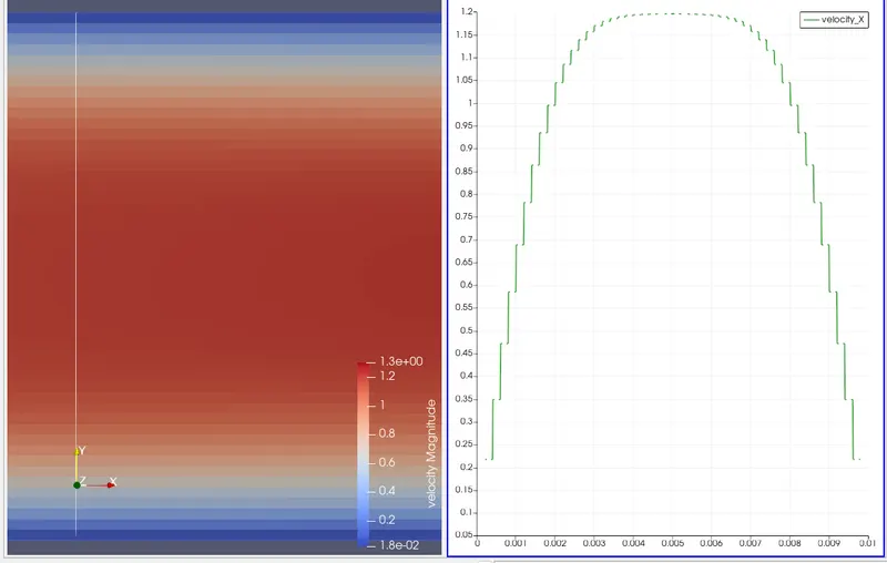
CASE2 MESH SIZE 1.5e-4

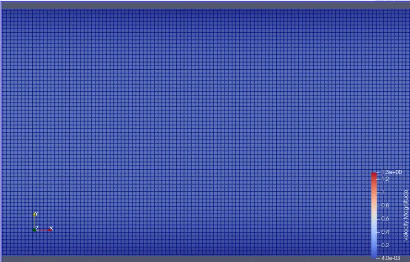
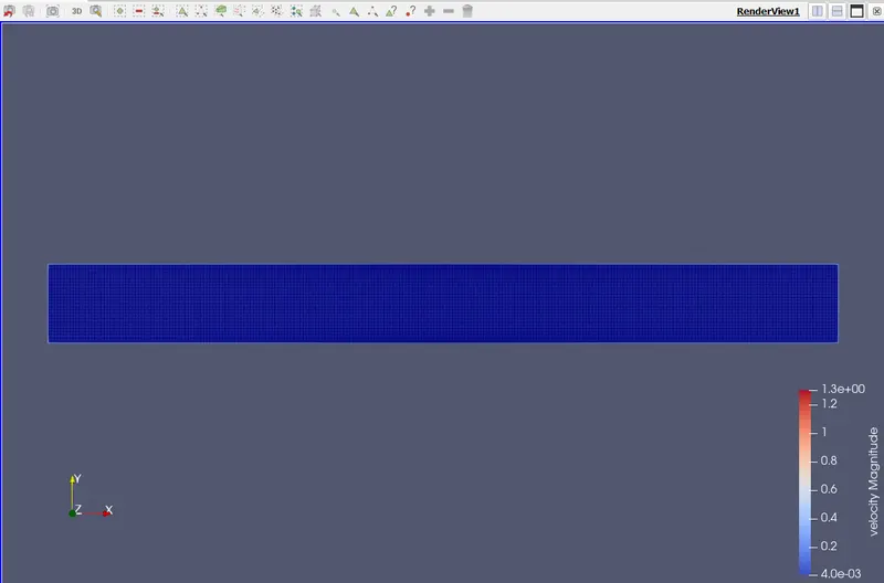
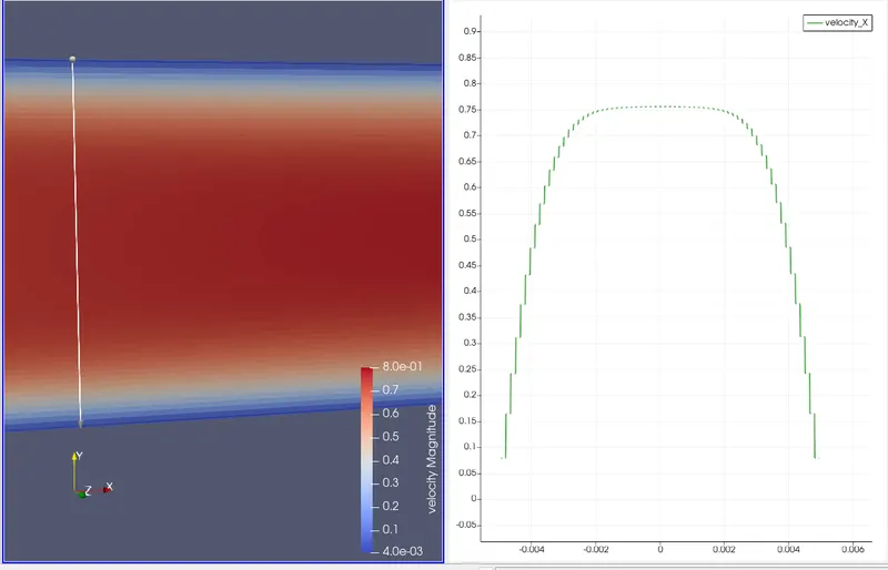
CASE3 MESH SIZE 1e-4

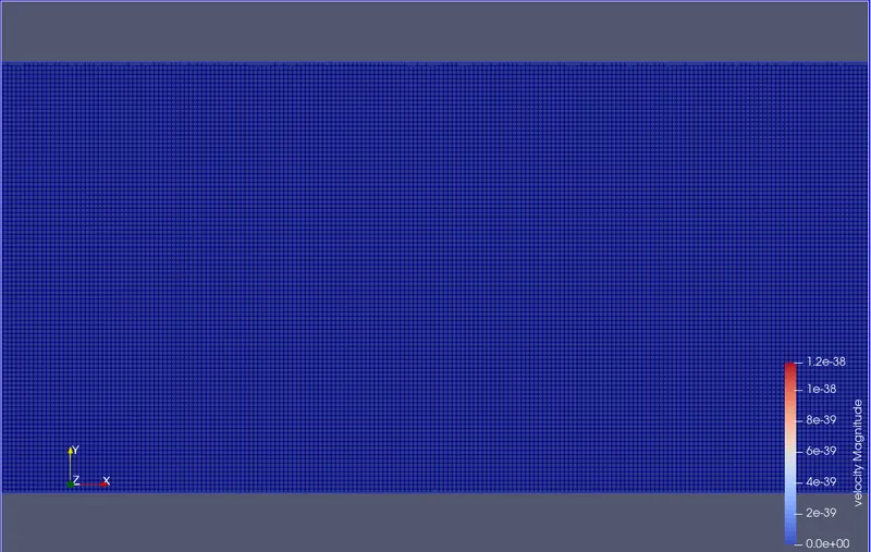
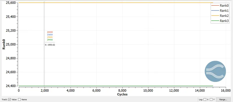
OBSERVATION:

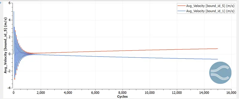
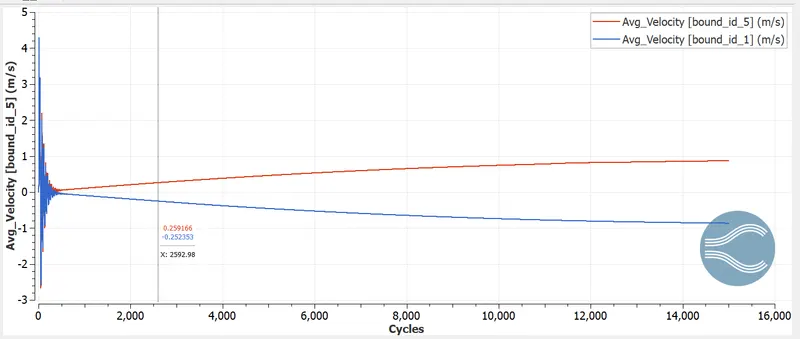
From the various plots of velocity contour we can say that at the entrance of the channel we have a flatter velocity profile but as we approach outlet we see much more parabolic profile.

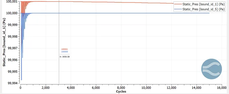
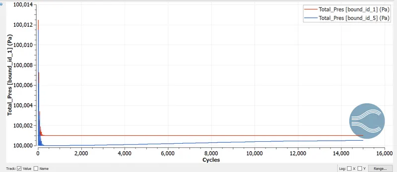
The flow in the channel is due to the pressure difference between inlet and outlet.

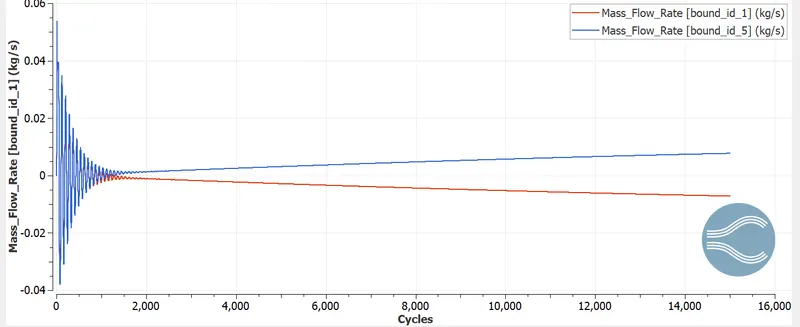
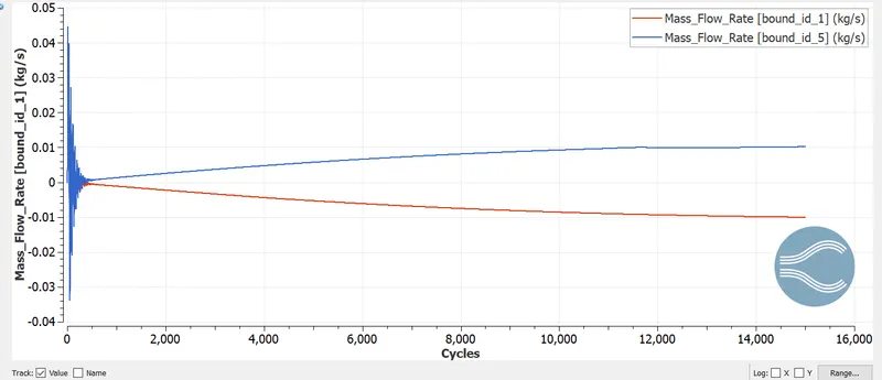
From the plots of mass flow rate at inlet and outlet we can conclude that the conservation of mass is happening in the system.

From the plots of stattic pressure we observe that pressure at outlet increases marginally as number of cycles are being computed.

With increase in mesh refinment we get more accurate results and more number of cells but the simulation time increases significantly.