Week 1: Channel flow simulation using CONVERGE CFD
Channel Flow:-
Channel flow is an internal flow in which fluid flow inside a confined volume and changes its states and flow structures while advancing in flow.
In this project, flow of air(O2 and N2) is considered for flow inside a rectangular pipe taking a 2D replica of it for easier analysis and computation.
Objective:-
- Setup Channel flow Simulation
- Changing grid size to obtain finer Mesh for 3 different values
- Plot Velocity and Pressure contour for all 3 Meshes and obtaining Animation out of it.
Procedure:-
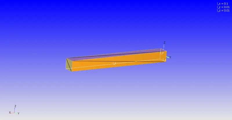
Geometry was made using Create command in side panel
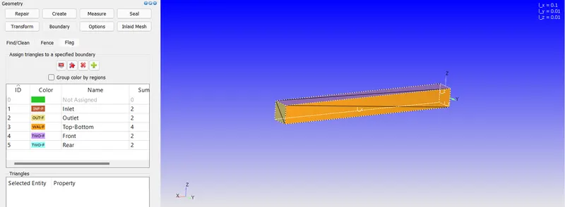
Boundary was made using Boundary tab available in side bar option
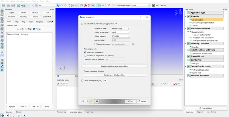
Gas Characteristics value was validated as by default value
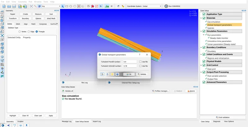
Global Transport properties was validated as by default value
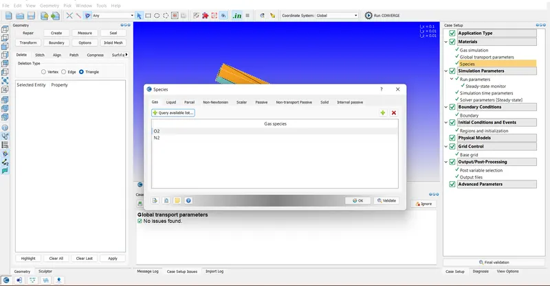
Two species named O2 and N2 was added from the list
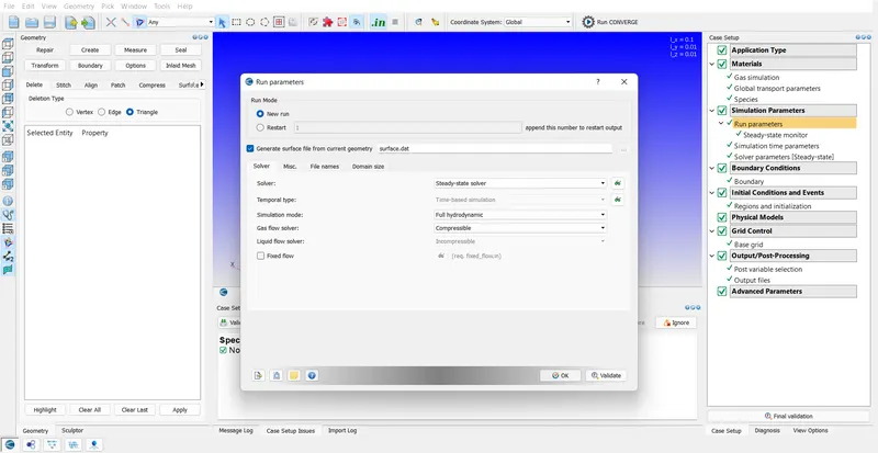
Run Parameters as Steady state solver with full hydronynamics was choosen
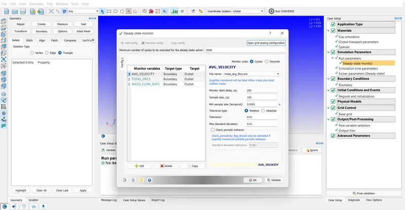
To monitor the progress in each span of time and lessening the simulation time Steady State monitor value was specified
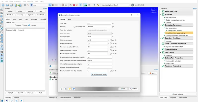
Simualtion time was set with end time as 15000 cycles with both the time steps as 1e-9 and maximum time step as 1
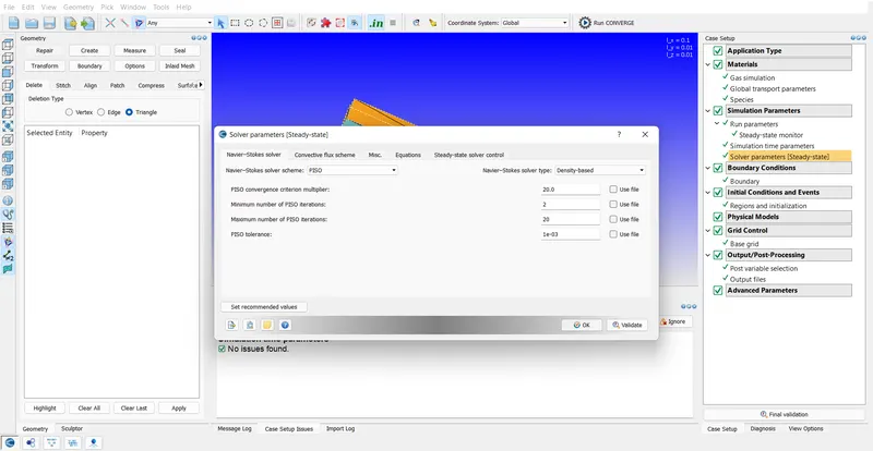
Solver Parameter was validated as the default value
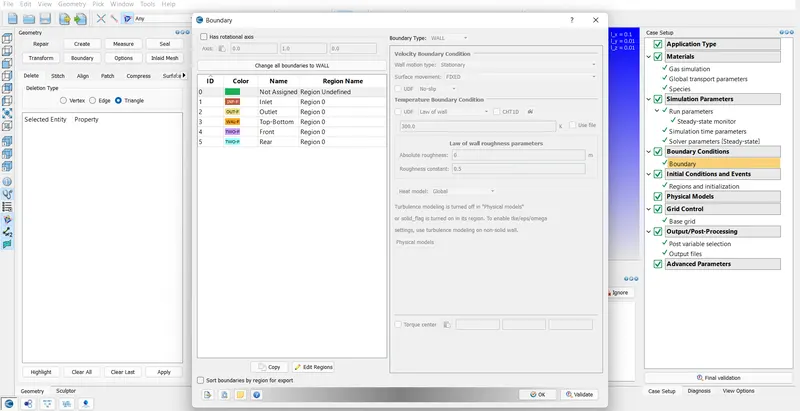
Boundary conditions and specified regions were alloted
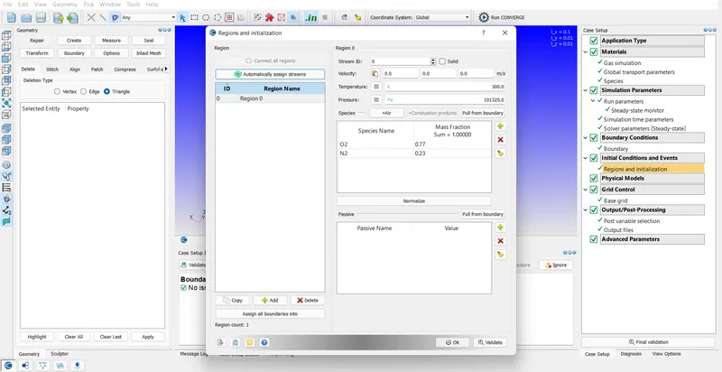
One regions was specified with exchanging the mass fraction of N2 and O2
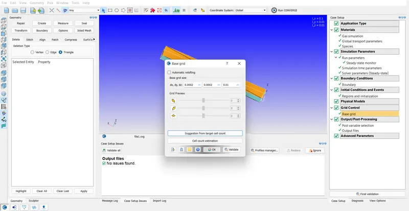
Three different Base Grid were specified for 3 different simulations
All the required post processing values were selcted vefore starting the simulation
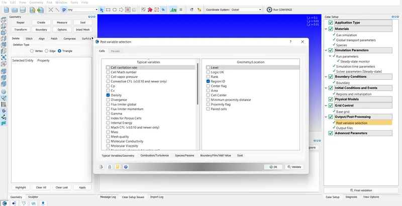
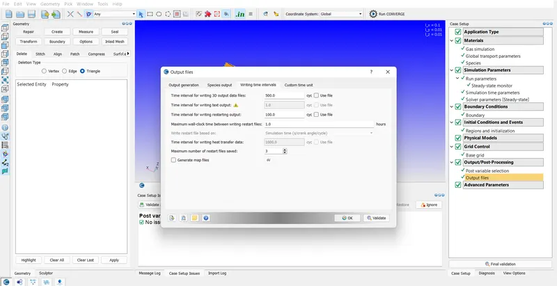
For better visualization and animation 1 writing file per 500 cycles were selected so that 300 output files will be obtained and for safety purpose 3 restart files were saved with 100 cycles as time interval for writing new file
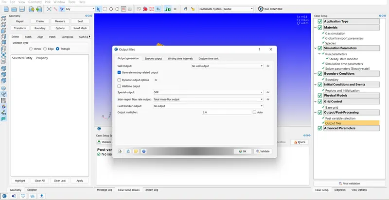
In output generation tab all the parameters were set by default
Obsevations:-
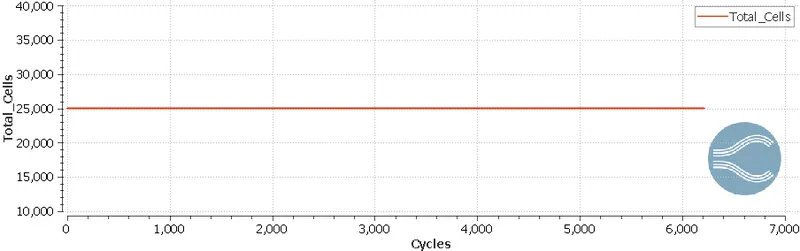
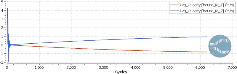
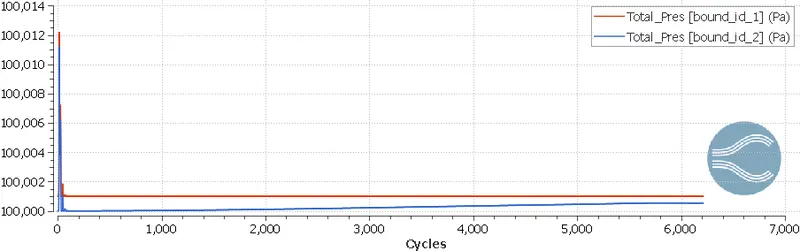
i)Base Grid:2e-4
Mesh
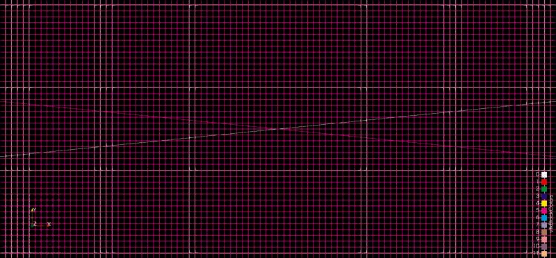
Total Cell Count
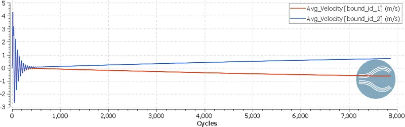
Average Velocity
Total Pressure
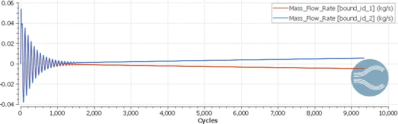
Mass Flow Rate
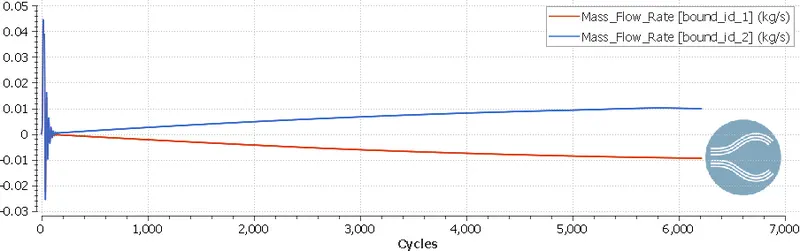
ii)Base Grid: 1.5e-4
Base Grid
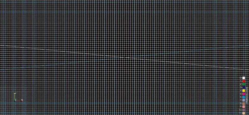
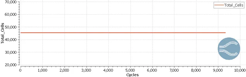
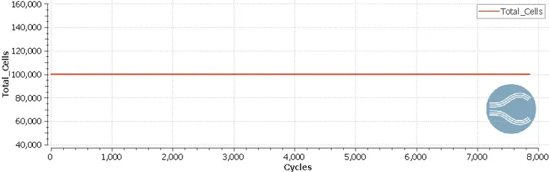
Total Cell Count
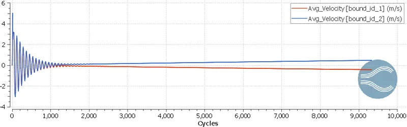
Average Velocity
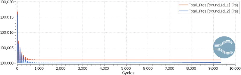
Total Pressure
Mass Flow Rate
iii)Base Grid: 1e-4
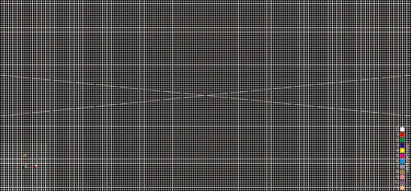
Mesh
Total Cell Count
Average Velocity
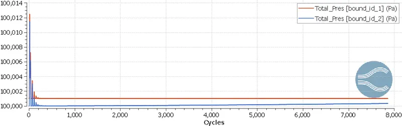
Total Pressure
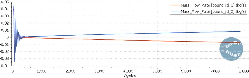
Mass Flow Rate
Contour Plot:-
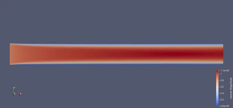
Velocity Contour
2e-4 Base Grid
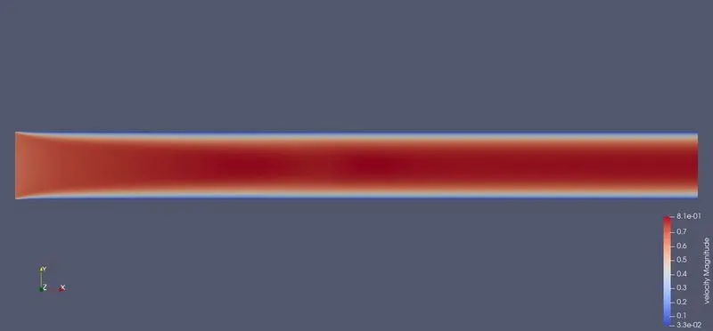
1e-4 Base Grid
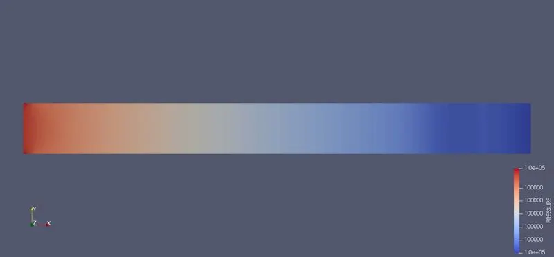
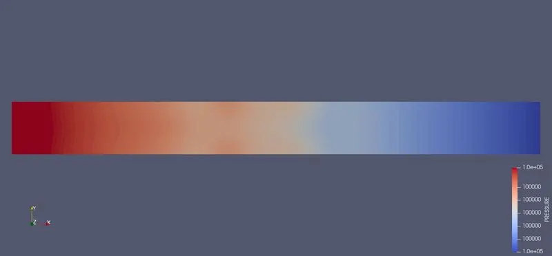
Pressure Contour
2e-4 Base Grid
1e-4 Base Grid
Animation Video:-
Pressure Contour
Velocity Contour
Conclusion:-
- Finer the mesh accurate the result which can be quantified from the Plot Contour
- Cell counts for 2e-4,1.5e-4 and 1e-4 is 25000, 45000 and 100000 respectively
- As the velocity increased towards end of the flow the Pressure decreased
- Intial turbulance ended at a laminar flow
- Simulation time increased with increase in Mesh density
- Parallel processing with CYGWIN reduces simulation time as comapred to serial processing using a single processor
- It is a good idea to limit the number of cycles by giving minimum number cycles so that if converges before the entire cycle we can reduce the computation time hence increase the productivity and efficiency