Week 3.5 - Deriving 4th order approximation of a 2nd order derivative using Taylor Table method

Objective:- To find 4th order approximations of the second order derivative using:-

1. Central Differencing
2. Skewed right-sided differencing
3. Skewed left-sided differencing

Using central differencing method the equation becomes:-

`(del^2u)/dx^2=(af(i-2)+bf(i-1)+cf(i)+df(i+1)+ef(i+2))/(Deltax^2)`

where,

a=-0.083333

b=1.333333

c=-2.500000

d=1.333333

e=-0.083333

function err_central_diff= central_diff(x,dx)
analytical_derivative=-2*exp(x)*sin(x);

a=-0.083333;
b=1.333333;
c=-2.500000;
d=1.333333;
e=-0.083333;

err_central_diff=abs((((a*exp(x-2*dx)*cos(x-2*dx))+(b*exp(x-dx)*cos(x-dx))+(c*exp(x)*cos(x))+(d*exp(x+dx)*cos(x+dx))+(e*exp(x+2*dx)*cos(x+2*dx)))/dx^2)-analytical_derivative);
end

Using right-skewed differencing method the equation becomes:-

`(del^2u)/dx^2=(af(i)+bf(i+1)+cf(i+2)+df(i+3)+ef(i+4)+gf(i+5))/(Deltax^2)`

a=3.75000

b=-12.83333

c=17.83333

d=-13.00000

e=5.08333

g=-0.83333

function err_skewed_right= right_diff(x,dx)
analytical_derivative=-2*exp(x)*sin(x);

a=3.75000;
b=-12.83333;
c=17.83333;
d=-13.0000;
e=5.08333;
g=-0.83333;

err_skewed_right=abs((((a*exp(x)*cos(x))+(b*exp(x+dx)*cos(x+dx))+(c*exp(x+2*dx)*cos(x+2*dx))+(d*exp(x+3*dx)*cos(x+3*dx))+(e*exp(x+4*dx)*cos(x+4*dx))+(g*exp(x+5*dx)*cos(x+5*dx)))/dx^2)-analytical_derivative);
end

Using right-skewed differencing method the equation becomes:-

`(del^2u)/dx^2=(af(i-5)+bf(i-4)+cf(i-3)+df(i-2)+ef(i-1)+gf(i))/(Deltax^2)`

a=-0.83333

b=5.08333

c=-13.00000

d=17.83333

e=-12.83333

g=3.75000

function err_skewed_left= left_diff(x,dx)
analytical_derivative=-2*exp(x)*sin(x);

g=3.75000;
e=-12.83333;
d=17.83333;
c=-13.0000;
b=5.08333;
a=-0.83333;

err_skewed_left=abs((((a*exp(x-5*dx)*cos(x-5*dx))+(b*exp(x-4*dx)*cos(x-4*dx))+(c*exp(x-3*dx)*cos(x-3*dx))+(d*exp(x-2*dx)*cos(x-2*dx))+(e*exp(x-dx)*cos(x-dx))+(g*exp(x)*cos(x)))/dx^2)-analytical_derivative);
end

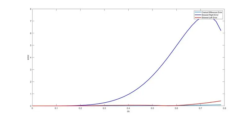
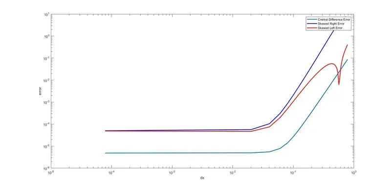
The below code is going to call the above function by passing the value of x and dx and plots the required figure:-

close all
clc

x=pi/3;
dx=linspace(pi/4,pi/40000,40);

for i=1:length(dx)
    central_err(i)=central_diff(x,dx(i));
    right_err(i)=right_diff(x,dx(i));
    left_err(i)=left_diff(x,dx(i));
end

figure(1)
plot(dx,central_err,'linewidth',2)
hold on
plot(dx,right_err,'b','linewidth',2)
hold on
plot(dx,left_err,'r','linewidth',2)
xlabel('dx')
ylabel('error')
legend('Cnetral Difference Error', 'Skewed Right Error','Skewed Left Error')

figure(2)
loglog(dx,central_err,'linewidth',2)
hold on
loglog(dx,right_err,'b','linewidth',2)
hold on
loglog(dx,left_err,'r','linewidth',2)
xlabel('dx')
ylabel('error')
legend('Cnetral Difference Error', 'Skewed Right Error','Skewed Left Error')

Output Plot:-

Conclusion:-

Analysing the plots we can conclude that the best solution is given by Central differencing Method.

But, Skewed differencing is also useful when it comes it analysis in a boundary where we cant take initial inputs from both the side and it will give a reasonably acceptable output.