Week 7 - Simulation of a 1D Super-sonic nozzle flow simulation using Macormack Method
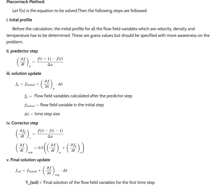
Objective:- To simulate the isoentropic flow through a quasi 1D subsonic-supersonic nozzle using both conservative and non-conservative forms and solving them using MacCormak's technique
Governing Equations:
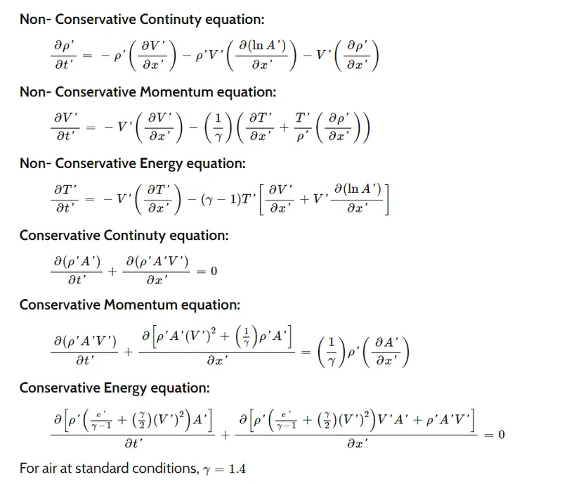
Conservative Function:-
function [mfr_nc,mfr_throat_nc]=non_conservative(L,n,nt,cfl)

x=linspace(0,L,n);
dx=x(2)-x(1);

rho=1-0.3146*x;
T=1-0.2314*x;
v=(0.1+1.09*x).*T.^0.05;
a=1+2.2*(x-1.5).^2;
M=v./(T.^0.5);
mfr=rho.*a.*v;
p=rho.*T;
g=1.4;

for z=1:31
    u=(T(z))^(1/2);
    dt(z)=cfl*dx/(u+v(z));
end
dt=min(dt);

for i =1:length(nt)
    rho_old=rho;
    T_old=T;
    v_old=v;
    for j=2:n-1
        drhodx=(rho(j+1)-rho(j))/dx;
        dvdx=(v(j+1)-v(j))/dx;
        dTdx=(T(j+1)-T(j))/dx;
        dadx=(log(a(j+1))-log(a(j)))/dx;
        drhodt_p(j)=-rho(j)*dvdx-rho(j)*v(j)*dadx-v(j)*drhodx;
        dvdt_p(j)=-v(j)*dvdx-(1/g)*(dTdx+(T(j)/rho(j))*drhodx);
        dTdt_p(j)=-v(j)*dTdx-(g-1)*T(j)*(dvdx+v(j)*dadx);

        v(j)=v_old(j)+dvdt_p(j)*dt;
        rho(j)=rho_old(j)+drhodt_p(j)*dt;
        T(j)=T_old(j)+dTdt_p(j)*dt;

        drhodx=(rho(j)-rho(j-1))/dx;
        dvdx=(v(j)-v(j-1))/dx;
        dTdx=(T(j)-T(j-1))/dx;
        dadx=(log(a(j))-log(a(j-1)))/dx;
        drhodt_c(j)=-rho(j)*dvdx-rho(j)*v(j)*dadx-v(j)*drhodx;
        dvdt_c(j)=-v(j)*dvdx-(1/g)*(dTdx+(T(j)/rho(j))*drhodx);
        dTdt_c(j)=-v(j)*dTdx-(g-1)*T(j)*(dvdx+v(j)*dadx);
    end

        drhodt_avg=0.5*(drhodt_p+drhodt_c);
        dvdt_avg=0.5*(dvdt_p+dvdt_c);
        dTdt_avg=0.5*(dTdt_p+dTdt_c);

    for j=2:n-1
        v(j)=v_old(j)+dvdt_avg(j)*dt;
        rho(j)=rho_old(j)+drhodt_avg(j)*dt;
        T(j)=T_old(j)+dTdt_avg(j)*dt;
    end


        v(1)=2*v(2)-v(3);

        v(n)=2*v(n-1)-v(n-2);
        rho(n)=2*rho(n-1)-rho(n-2);
        T(n)=2*T(n-1)-T(n-2);

        p=rho.*T;
        M=v./T.^0.5;
        mfr=rho.*a.*v;

        T_throat(i)=T(16);
        rho_throat(i)=rho(16);
        v_throat(i)=v(16);
        M_throat(i)=M(16);
        p_throat(i)=p(16);
        mfr_throat(i)=mfr(16);

        for ii=[1:50:201 700]
            if ii==i
                figure(1)
                plot(x,mfr,'linewidth',1)
                hold on
                title('Non-Conservative form - Variation of mass flow rate distribution inside the nozzle at different time steps')
                xlabel('Length of nozzle')
                ylabel('Mass flow rate')
            elseif i==1400
                plot(x,mfr,'*r')
                legend('@1','@51','@101','@151','@201','@700','@1400')
            end
        end
end
    if n==31
        figure(2)
        plot(x,v,'b',x,p,'r',x,T,'k',x,rho,'m',x,M,'g',x,mfr,'c')
        ylim([-0.1 3.7])
        title(sprintf('Timestep = %d',i))
        xlabel('Length of nozzle')
        ylabel('Non dimensional parameters')
        legend('Velocity','Pressure','Temperature','Density','Mach Number','Mass Flow Rate')
        title('Non- Conservative form- steady state variation of primitive variables inside the nozzle')

        figure(3)
        plot(i,rho_throat)
        hold on
        plot(i,v_throat,'linewidth',1.5)
        plot(i,p_throat,'linewidth',1.5)
        plot(i,T_throat,'linewidth',1.5)
        plot(i,M_throat,'linewidth',1.5)
        plot(i,mfr_throat,'linewidth',1.5)
        xlabel('Non dimensional parameters')
        legend('Velocity','Pressure','Temperature','Density','Mach Number','Mass Flow Rate')
        title('Non- Conservative form- time wise variation of primitive variables at the troat point i = 16')
    end
    mfr_nc=mfr;
    mfr_throat_nc=mfr_throat;
end
Non-Conservative Function:-
function [mfr_c,mfr_throat_c]=conservative(L,n,nt,cfl)

x=linspace(0,L,n);
dx=x(2)-x(1);

for ii=1:length(x)
    if (x(ii)<=0.5)
        rho(ii)=1;
        T(ii)=1;
    elseif (x(ii)>0.5) && (x(ii)<=1.5)
        rho(ii) = 1-0.366*(x(ii)-0.5);
        T(ii)=1-0.167*(x(ii)-0.5);
    elseif (x(ii)>1.5) && (x(ii)<=3.5)
        rho(ii) = 0.634-0.3879*(x(ii)-0.5);
        T(ii)=0.833-0.3507*(x(ii)-0.5);
    end
end

a=1+2.2*(x-1.5).^2;
g=1.4;
u1=rho.*a;
u2=0.59*ones(1,n);
v=u2./u1;
u3=u1.*((T./(g-1))+(g/2).*v.^2);
M=v./(T.^0.5);
mfr=rho.*a.*v;
p=rho.*T;

for z=1:31
    u=(T(z))^(1/2);
    dt(z)=cfl*dx/(u+v(z));
end
dt=min(dt);

for i=1:length(nt)
    u1_old=u1;
    u2_old=u2;
    u3_old=u3;

    for j=2:n-1

        f1=u2;
        f2=u2.^2./u1+((g-1)/g).*(u3-(g/2)*u2.^2./u1);
        f3=g.*u2.*u3./u1-0.5*g*(g-1).*u2.^3./u1.^2;

        j1=(1/g)*(rho(j)*T(j)*(a(j+1)-a(j))/dx);

        du1dt_p(j)=-(f1(j+1)-f1(j))/dx;
        du2dt_p(j)=-(f2(j+1)-f2(j))/dx+j1;
        du3dt_p(j)=-(f3(j+1)-f3(j))/dx;

        u1(j)=u1_old(j)+du1dt_p(j)*dt;
        u2(j)=u2_old(j)+du2dt_p(j)*dt;
        u3(j)=u3_old(j)+du3dt_p(j)*dt;

        rho=u1./1;
        T=(g-1).*(u3./u1-(g/2).*(u2./u1).^2);

        f1=u2;
        f2=u2.^2./u1+((g-1)/g).*(u3-(g/2)*u2.^2./u1);
        f3=g.*u2.*u3./u1-0.5*g*(g-1).*u2.^3./u1.^2;

        j2=(1/g)*(rho(j)*T(j)*(a(j)-a(j-1))/dx);

        du1dt_c(j)=-(f1(j+1)-f1(j))/dx;
        du2dt_c(j)=-(f2(j+1)-f2(j))/dx;
        du3dt_c(j)=-(f3(j+1)-f3(j))/dx;
    end

    du1dt_avg=0.5*(du1dt_p+du1dt_c);
    du2dt_avg=0.5*(du2dt_p+du2dt_c);
    du3dt_avg=0.5*(du3dt_p+du3dt_c);

    for k=2:n-1
        u1(k)=u1_old(k)+du1dt_avg(k)*dt;
        u2(k)=u2_old(k)+du2dt_avg(k)*dt;
        u3(k)=u3_old(k)+du3dt_avg(k)*dt;
    end
    u1(1)=a(1);
    u2(1)=2*u2(2)-u2(3);
    u3(1)=u1(1)*(T(1)/(g-1)+ (g*(u2(1)/u1(1))^2)/2);

    u1(n)=2*u1(n-1)-u1(n-2);
    u2(n)=2*u2(n-1)-u2(n-2);
    u3(n)=2*u3(n-1)-u3(n-2);

    rho=u1./a;
    v=u2./u1;
    T=(g-1).*(u3./-(g/2).*(u2./u1).^2);
    p=rho.*T;
    M=v./T.^0.5;
    mfr=u2;

    T_throat(i)=T(16);
    rho_throat(i)=rho(16);
    v_throat(i)=v(16);
    M_throat(i)=M(16);
    p_throat(i)=p(16);
    mfr_throat(i)=mfr(16);

    for ii=[1:50:201 700]
        if ii==i
            figure(4)
            plot(x,mfr,'linewidth',1)
            hold on
            title('Conservative form - Variation of mass flow rate distribution inside the nozzle at different time steps')
            xlabel('Length of nozzle')
            ylabel('Mass flow rate')
        elseif i==1400
            plot(x,mfr,'*r')
            legend('@1','@51','@101','@151','@201','@700','@1400')
        end
    end
end

    if n==31
        figure(5)
        plot(x,v,'b',x,p,'r',x,T,'k',x,rho,'m',x,real(M),'g',x,mfr,'c')
        ylim([-0.1 3.7])
        title(sprintf('Timestep = %d',i))
        xlabel('Length of nozzle')
        ylabel('Non dimensional parameters')
        legend('Velocity','Pressure','Temperature','Density','Mach Number','Mass Flow Rate')
        title('Conservative form- steady state variation of primitive variables inside the nozzle')

        figure(6)
        plot(nt,rho_throat)
        hold on
        plot(nt,v_throat,'linewidth',1.5)
        plot(nt,p_throat,'linewidth',1.5)
        plot(nt,T_throat,'linewidth',1.5)
        plot(nt,real(M_throat),'linewidth',1.5)
        plot(nt,mfr_throat,'linewidth',1.5)
        xlabel('Non dimensional parameters')
        legend('Velocity','Pressure','Temperature','Density','Mach Number','Mass Flow Rate')
        title('Non- Conservative form- time wise variation of primitive variables at the troat point i = 16')
    end
    mfr_c=mfr;
    mfr_throat_c=mfr_throat;
end
Main Calling Function:-
close all
clc

L=3;
n=[31 62 93];
nt=1:1400;
cfl=0.5;
for i=1:length(n)
    x=linspace(0,L,n(i));
    [mfr_nc,mfr_throat_nc]=non_conservative(L,n(i),nt,cfl);
    [mfr_c,mfr_throat_c]=conservative(L,n(i),nt,cfl);

    figure(7)
    subplot(2,1,1)
    plot(nt,mfr_throat_c,'b',nt,mfr_throat_nc,'r','linewidth',1.5)
    xlabel('Time steps (nt)')
    ylabel('Mass flow rate')
    legend('Conservation form','Non-Conservative form')
    title('Mass flow rate using "Non- Conservative form vs Conservative form " at throat point i=16')
    subplot(2,1,2)
    plot(x,mfr_c,'b',x,mfr_nc,'r','linewidth',1.5)
    xlabel('Length of nozzle')
    ylabel('Mass flow rate')
    legend('Conservation form','Non-Conservative form')
    title('Mass flow rate using "Non- Conservative form vs Conservative form " in the nozzle')

    figure(8)
    subplot(2,1,1)
    plot(nt,mfr_throat_c,'linewidth',1.5)
    hold on
    xlabel('Time steps (nt)')
    ylabel('Mass flow rate')
    legend('@31 nodes','@62 nodes','@93 nodes')
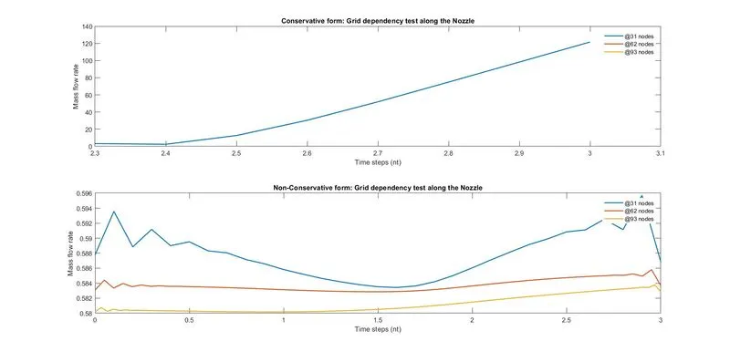
    title('Conservative form: Grid dependency test at throat point i =16')
    subplot(2,1,2)
    plot(nt,mfr_throat_nc,'linewidth',1.5)
    hold on
    xlabel('Time steps (nt)')
    ylabel('Mass flow rate')
    legend('@31 nodes','@62 nodes','@93 nodes')
    title('Non-Conservative form: Grid dependency test at throat point i =16')

    figure(9)
    subplot(2,1,1)
    plot(x,mfr_c,'linewidth',1.5)
    hold on
    xlabel('Time steps (nt)')
    ylabel('Mass flow rate')
    legend('@31 nodes','@62 nodes','@93 nodes')
    title('Conservative form: Grid dependency test along the Nozzle')
    subplot(2,1,2)
    plot(x,mfr_nc,'linewidth',1.5)
    hold on
    xlabel('Time steps (nt)')
    ylabel('Mass flow rate')
    legend('@31 nodes','@62 nodes','@93 nodes')
    title('Non-Conservative form: Grid dependency test along the Nozzle')
end
Figure 1
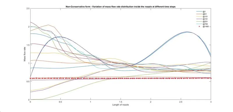
Figure 2
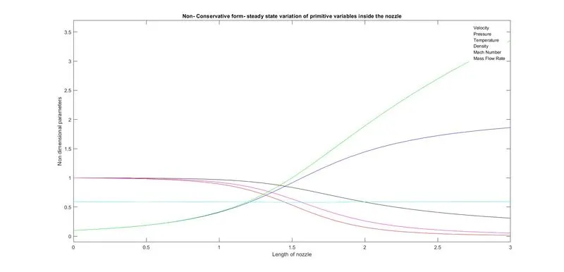
Figure 4
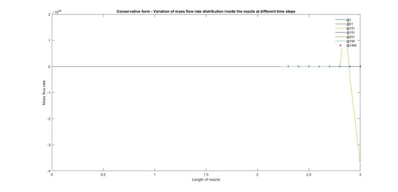
Figure 5
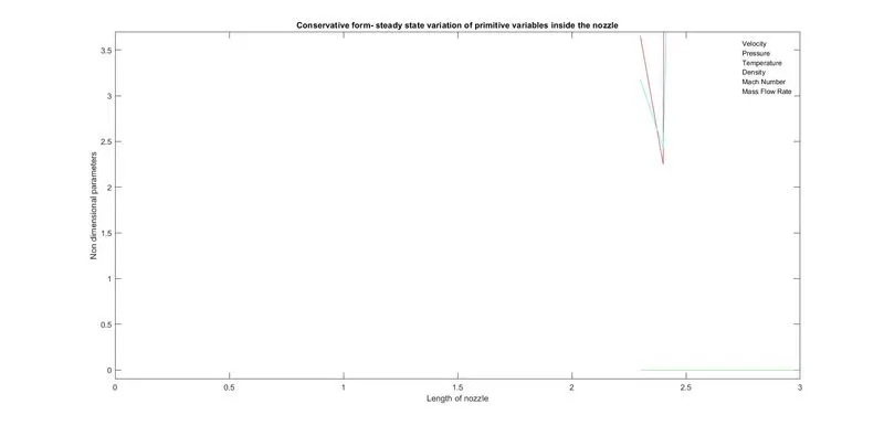
Figure 6
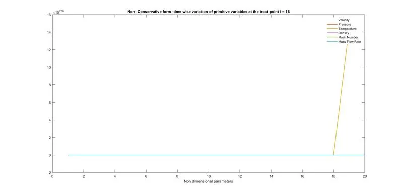
Figure 7
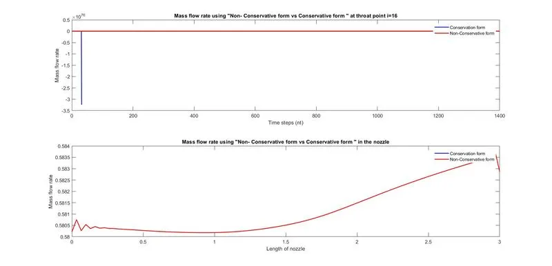
Figure 8
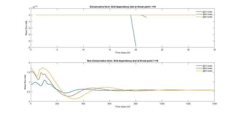
Figure 9