Understanding the stability analysis

Aim: The main goal of this challenge is to solve the given set of linear equations using iterative methods and study the convergence rate by varying Spectral Radius. By changing the spectral radius, we observe its effect on the system and its stability.

• Objectives:

  1. Arrange the given set of linear equations into a system of Matrices.
  2. Solve the system of Matrices using Jacobi, Gauss-Seidel and SOR methods.
  3. Calculate the Iteration Matrix for all the iterative methods.
  4. Calculate the Eigen Value and the Spectral Radius of the Iteration Matrix.

5.study the convergence rate by varying the Spectral Radius.

Given Data:

A=[5 1 2 ; -3 9 4; 1 2 -7]

X=[x1;x2;x3]

B=[10 -14 33]

Let us now state the given set of linear equations:

`5x_1 + x_2 + 2x_3 = 10`

`-3x_1 + 9x_2 + 4x_3 = -14`

`x_1 + 2x_2 -7x_3 = 33`

Writing the above equations in the matrix form:

This is in the form `AX = B`

`[[5,1,2],[-3,9,4],[1,2,-7]] * [[x_1],[x_2],[x_3]] = [[10],[-4],[33]]`

where `A = [[5,1,2],[-3,9,4],[1,2,-7]]`

`X = [[x_1],[x_2],[x_3]]` and

`B = [[10],[-4],[33]]`

Now, we have to decompose matrix A into its Lower, Upper and Diagonal matrices.

`U = [[0,1,2],[0,0,4],[0,0,0]]`

`L = [[0,0,0],[-3,0,0],[1,2,0]]`

`D = [[5,0,0],[0,9,0],[0,0,-7]]`

Jacobi Method:

We use the following equation in a loop until convergence is achieved in order to solve the unknowns:

`X^(n+1) = (D^-1) * (B - D^-1) * ((L + U) * x^(n))`

The following equation is used to calculate the Iteration Matrix in Jacobi Method:

`T_(iteration) = D^(-1) * (L + U)`

Gauss-Seidel Method:

We use the following equation in a loop until convergence is achieved in order to solve the unknowns:

`X^(n+1) = (D + L)^-1 * (B - (L + D)^-1) * U * X^n`

The following equation is used to calculate the Iteration Matrix in Gauss-Seidel Method:

`T^(iteration) = (D+L)^-1 * U`

Successive Over Relaxation Method:

We use the following equation in a loop until convergence is achieved in order to solve the unknowns:

`X^(n+1) = ((D+(omega*L)^-1))*((omega*B)-(((omega*U)-((1-omega)*D))*x^n))`

The following equation is used to calculate the Iteration Matrix in SOR Method

`T^(iteration) = (D + (omega*L))^-1 * ((1 - omega) * D + (omega * U))`

Where, D = Diagonal Matrix.

L = Lower Diagonal Matrix.

U = Upper Diagonal Matrix.

ω = relaxaton factor.

MATLAB CODE:

MAIN CODE:

clear all
close all
clc

%inputs
A=[5 1 2; -3 9 4; 1 2 -7];
B=[10; -14; -33];

%Diagonal Matrix
D=[5 0 0; 0 9 0; 0 0 -7];

%Upper Diagonal Matrix
U=[0 1 2; 0 0 4; 0 0 0];

%Lower Diagonal Matrix
L=[0 0 0; -3 0 0; 1 2 0];

% Coefficient Matrix of A
A = D + L + U;
%RHS Matrix
B=[10 -14  33];

R =L+U;
%omega is relaxation  factor for sor.
w = 1.25;

magnifying_factor=linspace(0.5,5,10);


for i=1:length(magnifying_factor)
    D1 = magnifying_factor(i)*D;
    
    % Computing iteration matrix.
    T_jac = inv(D1)*(L+U);
    T_gs = inv(D1+L)*U;
    T_sor = inv(D1+w*L)*((1-w)*D1-w*U);
    
    % Computing eigen values of iteration matrix.
    eigenvalue_jac = roots(poly(T_jac));
    eigenvalue_gs = roots(poly(T_gs));
    eigenvalue_sor = roots(poly(T_sor));
     
    % Computing spectral radius of iteration matrix.
    %rho_jac = spectral_radius
    spectral_radius_jac(i) = max(abs(eigenvalue_jac));
    spectral_radius_gs(i) = max(abs(eigenvalue_gs ));
    spectral_radius_sor(i) = max(abs(eigenvalue_sor));
      
    % Calling iterative  method.
    [jacobi_iter(i), x_jac] = jacobi(D1,L,U,B);
    [gs_iter(i),x_gs] = gaussiedle(D1,L,U,B);  
    [sor_iter(i),x_sor] = sor(D1,L,U,B,w);
end   

% plotting

figure(1)
subplot(2,1,1)
hold all
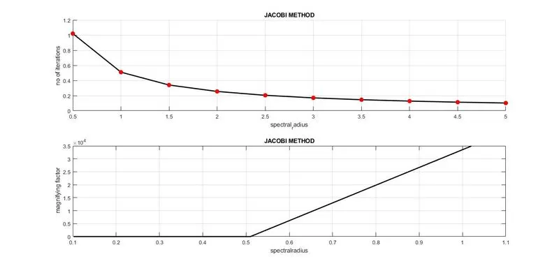
plot(magnifying_factor,spectral_radius_jac,'-o','markerfacecolor','r','markeredgecolor','r','color','k','linewidth',2)
xlabel('spectral_radius')
ylabel('no of iterations')
title('JACOBI METHOD')
grid on
subplot(2,1,2)
plot(spectral_radius_jac,jacobi_iter,'color','k','linewidth',2)
xlabel('spectralradius')
ylabel(' magnifying factor')
title('JACOBI METHOD')
grid on


figure(2)
subplot(2,1,1)
hold all
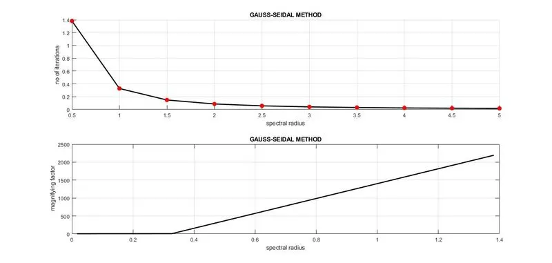
plot(magnifying_factor,spectral_radius_gs,'-o','markerfacecolor','r','markeredgecolor','r','color','k','linewidth',2)
ylabel('no of iterations')
xlabel('spectral radius')
title('GAUSS-SEIDAL METHOD')
grid on
subplot(2,1,2)
plot(spectral_radius_gs,gs_iter,'color','k','linewidth',2)
xlabel('spectral radius')
ylabel(' magnifying factor')
title('GAUSS-SEIDAL METHOD')
grid on


figure(3)
subplot(2,1,1)
hold all
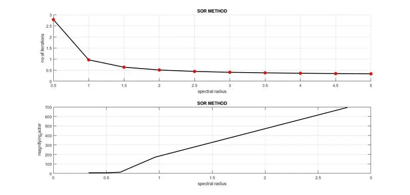
plot(magnifying_factor,spectral_radius_sor,'-o','markerfacecolor','r','markeredgecolor','r','color','k','linewidth',2)
xlabel('spectral radius')
ylabel('no of iterations')
title('SOR METHOD')
grid on
subplot(2,1,2)
plot(spectral_radius_sor,sor_iter,'color','k','linewidth',2)
xlabel('spectral radius')
ylabel(' magnifying_factor')
title('SOR METHOD')
grid on

Code for Jacobi function:

function [jacobi_iter,x_jac] = jacobi(D,L,U,B)
error = 9e9;
R = L+U;
tol = 1e-3;
x=[0;0;0];
xold=x;


jacobi_iter = 0;
  while (error>tol)
      x_jac = inv(D)* (B-(R*xold));
      error = max(abs(x_jac-xold));
      xold = x_jac;
      jacobi_iter=jacobi_iter+1;
  end    
end      

Code for Gauss-seidal function:

function [gs_iter,x_gs] = gaussiedle(D,L,U,B);
error = 9e9;
%R = L+U;
tol = 1e-3;
x=[0;0;0];
xold=x;

gs_iter = 1;
  while (error>tol)
      x_gs = (inv(D+L))*(B-(U*xold));
      error = max(abs(x_gs-xold));
      
      xold = x_gs;
      gs_iter = gs_iter +1;
  end    
end      

Code for SOR function:

function [sor_iter,x_sor] = sor(D,L,U,B,w);
error = 9e9;
tol = 1e-3;
x=[0;0;0];
xold=x;
sor_iter = 1;
  while (error>tol)
      %x_sor = inv(D-w*L)*((1-w)*D+w*U)*xold*inv(D-w*L)*B;
      x_sor = inv(D+w*L)*((w*B) - (w*U*xold)-((w-1)*D*xold));
      error = max(abs(x_sor-xold));
      xold = x_sor;
      sor_iter = sor_iter +1;
  end    
end      

Plot for Jacobi function:

Plot for Gauss-seidal function:

Plot for SOR function:

Results:-

1. The above plotted graphs show the comparision of a spectral radius vs number of iterations and spectral radius vs magnifying factor. The above comparision s done by three iterative techniques i.e. jacobi, gauss-sedal and SOR methods.
2. It is observed that on increasing the spectral radius, the number of iteratons requred for convergence also increases. Hence spectral radius is directly praportional to number of iterations.
3. From spectral radius vs magnifying factor plots, it is concluded that on increasng the magnifying factor the spectral radius decreases. Hence spectral radius is inversly praportional to the magnifying factor.
4. In general for the larger values of the diaognal entries,smaller wll be the spectral radius.
5. If the spectral radius goes above 1, the matrx is unsolvable with the iterative techniques.