Linear Convection for varying number of nodes

Objective:

Numerical solution to the Wave equation.

1. Assume that the domain length is L = 1m

2. The initial velocity profile is a step function. It is equal to 2m/s between x= 0.1 and 0.3 and 1m/s everywhere else.

3. Using first-order forward differencing for the time derivative.

4. Using first-order backward/rearward differencing for the space term.

5. Time step and number of grid points should be variables in your calculation

6. C = 1

7. Set time step = 0.01

Expected output

1. For C = 1 and for time = 0.4 seconds, comparing the original and final velocity profiles.

2. Make the comparison for n=20,40,80 and 160.

Aim: The main goal of this challenge is to solve the PDE 1Dimensional linear convection equation using MatLab and compare the effect grid size on the solution.

Formula of 1D linear convection:

`(delu)/(delt) = -C*(delu)/(delx)`

Matlab code:

close all
clear all
clc
L=1; %length of domain
n=input('number of nodes='); %the input should required number of nodes.
c=1; %convection velocity
x=linspace(0,L,n);
dx=L/(n-1);
x_start=0.1;
x_end=0.3;
n_start= round((x_start/dx)+1)
n_end=round((x_end/dx)+1)
%calculations
%Creating an array of u as per the given values
u=1*ones(1,n);
u(1)=1;
u(n_start:n_end)=2;
dt=0.01; %time step
% Boundry conditions
uold = u;
u_initial=u;
t=0.4;
ct=1;

%Time marching solution
nt=t/dt;
%time loop
for k=1:nt
% space loop
for i=2:n
%first order backward differencing for space term & forward differencing for time
u(i)= uold(i)-(c*dt/dx)*(uold(i)-uold(i-1));
end
uold=u;

%plotting the velocities
plot(x, u,'color', 'b')  % final velocity profile
hold on
grid on
plot(x,u_initial,'color', 'r');  % original velocity profile
axis([0 1 0 2]);
pause(0.04);
xlabel('Domain length');
ylabel('velocity');
legend('final velocity','initial velocity');
 
end

The above programe was executed at four different values of number of grid points, n=20, 40,80,160. This generated four graphs for linear convection and four videos were also generated.

Explanation :-

for this program number of grid points is defined as an array i.e. [20,40,80,160]. First declair all the necessary inputs for the linear convection problem including the number of grid points(array term). Time step is considered as the value of dt, hence time step (dt)=0.01. Initial velocity profile is given as a step function which is equal to 2m/s between x=0.1 and x=0.3 and rest 1m/s. size of domain is denoted by 'x'. where we use linspace() function in it to specify the interval. Grid size is equal to distance between their adjacent nodes. i.e. dx=L/(n(i)-1). Defining the 'x_start' & 'x_end' as o.1 and 0.3 respectively. and creating array at nodes for velocity is 1m/s as ' u = ones(1,n(i)) '. Now evaluate the nodes at the start & end for the various values of i. i.e. n_start(i) and n_end(i). Function ' round(a) ' and ' round(b) ' - here each element of a and b to th enearest integer value. same logic is used in the program. similarly defining the nodes at velocity is 2m/s i.e. " u(n_start(i): n_end(i)) = 2 ". As we know that t=0.4s and time step is dt the number of steps are calculated and alloted to variable- 'nt'. i.e time loop - " nt=t/dt ". There are nt -time steps a for loop is introduced to calculate the values it gives nt . Inside time loop space loop is created to calculate velocity at each node for each time step i.e from 2nd node to end node by backward differencing. After calculating the space loop immediately update old velocity term. Hence time step loop is then completely excutied. Then a final velocity profile is plotted on the same plot where the initial velocity profile is plotted for better comparision.

At node=20

https://youtu.be/gevlEqsWGcs

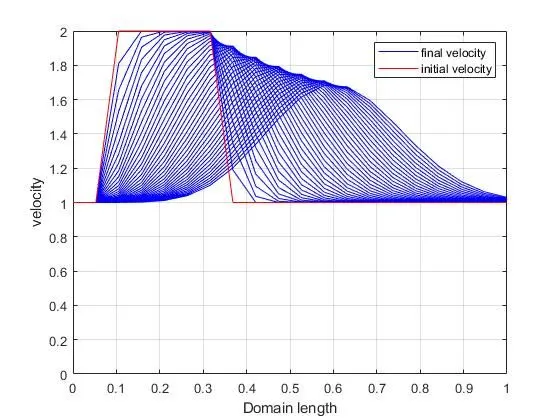
The above graph is generated at n=20. The velocity profile is moving from left to right.The red colour profile represents the original velocity profile and the blue colour profile is the final velocity profile. As the profile moves from left to right, it gets smoother and the peak value of velocity is continuously reducing.

At node=40

https://youtu.be/6veqML7RziA

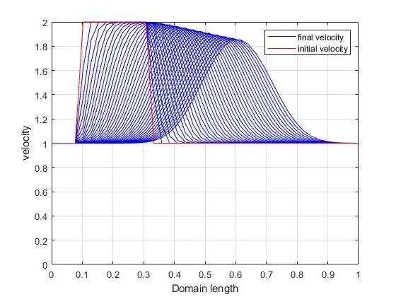
The above graph is generated at n=40. The velocity profile is moving from left to right.The red colour profile represents the original velocity profile and the blue colour profile is the final velocity profile.As compared to the first graph, this graph is less smoother and its peak velocity did not decreased drasticaly as it did in the first graph.

At node=80

https://youtu.be/O2bUI1drZmQ

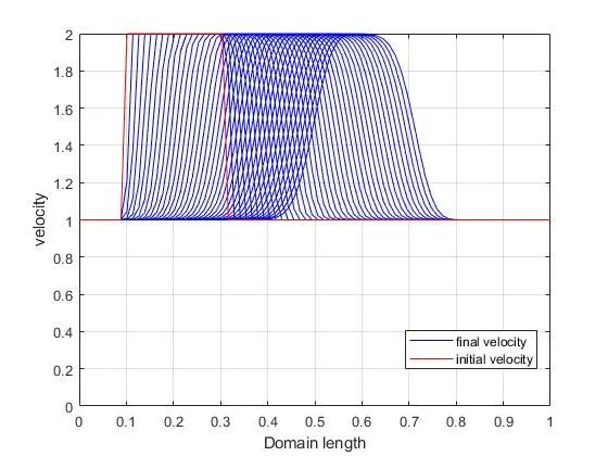
The above graph is generated at n=80. The velocity profile is moving from left to right. The red colour profile represents the original velocity profile and the blue colour profile is the final velocity profile. In this graph we observe that the sharpness of the square wave is maintained for a longer time as compared to the first two graphs. The paek value of the velocity is almost maintained till the final profile.

At node=160

https://youtu.be/U5QmYYKJ9Yw

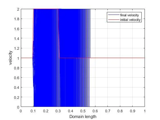
The above graph is generated at n=160. The velocity profile is moving from left to right. No square wave is generated in this graph. Here, we see a lot of wiggles and oscilations. The solution is ustable.

Conclusion:- Four graphs were generated at different number of grid points. At first the velocity profile bacome more stable and more squre wave with the increase in number of grid points from n=20 to n=80. But when we generated the profile at n=160 the solution was ustable, square wave profile was completely lost. This means there is a limit on how much finner grid we can use to find the solution. In general the finner the grid the better the solution will be, but there is a limit for finner grid after which the solution will be ustable.