Linear Convection for varying timesteps

Aim:

The main goal of this challenge is to solve the PDE 1Dimensional linear convection equation using MatLab for varying values of time steps and comparing the effect of the time step on the numerical solution.

Input conditions:

1. Number of nodes, n = 80

2. Time step , dt = 1e-4, 1e-3, 1e-2, and 1e-1

3. Simulation run time , t = 0.4 seconds.

Convection:

Convection is basically defined as the bulk movement of a fluid from one position to another with a particular velocity. An example of convection in fluids can be observed in the Navier-Stokes Equations which are given below.

`rho((delu)/(delt)+u(delu)/(delx)+u(delv)/(dely)) = -(delP)/(delx) + mu( (del^2u)/(delx^2)+(del^2u)/(dely^2))`

The above equation represents a simplified form of the Navier-Stokes Equation represented in two dimensions (x,y). Here, the spatial derivative terms of the velocity wrt. x and y are the convective terms.

Deriving a simple convection equation from the Navier-Stokes Equations,

`(delu)/(delt) + c(delu)/(delx) = 0`

where 'c' is a constant which denotes the speed of propagation.

The initial boundary conditions for the above equation are given as.

u(x=0,t=0) = 1m/s

c=1 m/s

The time derivative is approximated using a First Order Forward Differencing Scheme (to evaluate the velocity in the next time step), whereas the Space derivative is approximated using a Second Order Backward Differencing Scheme.

`(delu)/(delx) approx (u(x)-u(x-dx))/dx`

`therefore` the explicit equation for solving the 1D Convection is given as, `(u_i^(n+1) -u_i^n)/dt = c(u_i^n - u_(i-1)^n)/dx = 0`

On rearranging the terms,

`u_i^(n+1) = u_i^n - ((c**dt)/dx)(u_i^n-u_(i-1)^n)`

The above equation represents the "Explicit Solver" used to solve the convection equation.

CFL criteria that govern the linear convection equation:

The Courant–Friedrichs–Lewy or CFL condition is a condition for the stability of unstable numerical methods that model convection or wave phenomena. As such, it plays an important role in CFD.

What is CFL condition?

Culbert B. Laney’s definition of the CFL condition, from the book “Computational Gasdynamics”, is as follows: the full numerical domain of dependence must contain the physical domain of dependence. Therefore, the CFL condition expresses that the distance that any information travels during the timestep length within the mesh must be lower than the distance between mesh elements. In other words, information from a given cell or mesh element must propagate only to its immediate neighbors. The CFL condition is commonly confused with linear stability conditions or nonlinear stability conditions. However, it’s important to emphasize that it is not a sufficient condition for stability, and other stability conditions are generally more restrictive than the CFL condition.

CFL Derivation:

We can derive the CFL condition in a simple and intuitive way. Let’s begin by considering the simple linear convection problem of a quantity u:

For the simple problem of linear convection of a quantity u, the first order explicit upwind scheme becomes:

where a is the velocity magnitude, Δt is the timestep and Δx is the length between mesh elements.

By performing a Taylor series expansion on this scheme, this scheme introduces what is called a numerical diffusion, or numerical viscosity, equal to:

As expected from a diffusion coefficient, the numerical diffusion coefficient must be positive, otherwise, the solution will grow indefinitely with respect to time, making the numerical scheme unstable.

The right term inside the parenthesis of the above expression is commonly referred to as the Courant number, which is a dimensionless quantity. Therefore, the Courant number can be stated as follows:

It follows from the numerical diffusion coefficient discussion, that for any explicit simple linear convection problem, the Courant number must be equal or smaller than 1, otherwise, the numerical viscosity would be negative:

.

MATLAB Code for Main Function:

clear all
close all
clc

%Inputs for the Linear Convection Problem
L=1;    %Length of domain
n=80;   %No. of nodes
c=1;    %Convective Coefficient 
x=linspace(0,L,n);
dx=L/(n-1);
n_start = 0.1; %Given starting point of velocity
x_start= ((n_start/dx)+1);
n_end = 0.3;
x_end=((n_end/dx)+1);
u(x_start:x_end)=2;
u=1*ones(1,n);
u_old=u;
u_initial=u;
%Linear Convection for varying timesteps
%tic and toc are used to measure the elapsed time
 
%For time step dt=1e-1
tic
[u1,x1] = solution(1e-1);
simulation_time1=toc;

%For time step dt=1e-2
tic
[u2,x2]=solution(1e-2);
simulation_time2=toc;

%For time step dt=1e-3
tic
[u3,x3]=solution(1e-3);
simulation_time3=toc;

%For time step dt=1e-4
tic
[u4,x4]=solution(1e-4);
simulation_time4=toc;

%Plotting the results
%For timestep dt=1e-1
figure(1)
subplot(2,2,1)
plot(x1,u1,'k','linewidth',1);
hold on 
grid on 
plot(x,u_initial,'c','linewidth',1);
axis([0,1,0,2])
xlabel('Domain Length');
ylabel('Velocity (m/s)');
title('Linear Convection Velocity Profile for dt=1e-1');

%For time step dt=1e-2
subplot(2,2,2)
plot(x2,u2,'k','linewidth',1);
hold on
grid on 
plot(x,u_initial,'c','linewidth',1);
axis([0,1,0,2])
xlabel('Domain Length');
ylabel('Velocity (m/s)');
title('Linear Convection Velocity Profile for dt=1e-2');

%For time step dt=1e-3
subplot(2,2,3)
plot(x3,u3,'k','linewidth',1);
hold on 
grid on
plot(x,u_initial,'c','linewidth',1);
axis([0,1,0,2])
xlabel('Domain Length');
ylabel('Velocity (m/s)');
title('Linear Convection Velocity Profile for dt=1e-3');

%For time step dt=1e-4
figure(2)
subplot(2,2,1)
plot(x4,u4,'k','linewidth',1);
hold on 
grid on
plot(x,u_initial,'c','linewidth',1);
axis([0,1,0,2])
xlabel('Domain Length');
ylabel('Velocity (m/s)');
title('Linear Convection Velocity Profile for dt=1e-4');

%Plotting the comparison of velocity profiles for varying time steps
subplot(2,2,2)
plot(x1,u1,'k','linewidth',1);
hold on 
plot(x2,u2,'c','linewidth',1);
hold on
plot(x3,u3,'g','linewidth',1);
hold on
plot(x4,u4,'y','linewidth',1);
hold on 
grid on 
axis([0,1,0,2])
legend('dt=1e-1 ','dt=1e-2','dt=1e-3','dt=1e-4')
xlabel('Domain Length');
ylabel('Velocity (m/s)');
title('Comparison of Velocity Profiles for various time steps');

%Plot for Simulation time
subplot(2,2,3)
c = categorical({'dt=1e-1' 'dt=1e-2' 'dt=1e-3' 'dt=1e-4'});
simulation_time = [simulation_time1 simulation_time2 simulation_time3 simulation_time4]
grid on
bar(c,simulation_time);
xlabel('Time Steps');
ylabel('Simulation Time');
title('Simulation Time for various time steps dt');

MATLAB Code for 'Solution' Function to determine Velocity Profile for varying time steps:

function [u,x] = solution(dt)

%Inputs for the Linear Convection Problem
L=1;    %Length of the domain
n=80;   %No. of Grid Points - Subject to change (21,41,81,161)
c=1;    %Initial Velocity or Convective Coefficient 
x=linspace(0,L,n);
dx=x(2)-x(1);
u=1*ones(1,n);
n_start = 0.1; %Given starting point of velocity
x_start= ((n_start/dx)+1);
n_end = 0.3;
x_end=((n_end/dx)+1);
u(x_start:x_end)=2;
u_old=u;

t_final=0.4;
nt=t_final/dt;

for k=1:nt %Time Loop
    for i=2:n %Space Loop
        u(i)=u_old(i)-(c*dt/dx)*(u_old(i)-u_old(i-1));
    end
    u_old=u;
end

Main Script Explanation

• The command 'tic' and 'toc' are used to evaluate the time elapsed during simulation of the velocity profiles.
• The 'solution' function is called with the value of 'dt' as input to the function. It is used to evaluate the velocity profile at the particular time step value.
• The function is called 4 times with 4 varying values of 'dt' to evaluate the velocity profiles for varying time steps.
• Then, the plot code is written to compare the initial velocity with the final velocity profile obtained for a particular time step value 'dt'.
• Four plots comparing the initial and final velocity profiles for 4 different values of time steps are obtained.
• A final plot comparing the final velocity profiles for varying time steps is obtained.
• Then, to obtain the bar graph, the command 'categorical' is used to provide a sequence of order. Here, we have provided the various values of dt on the x axis.
• The 'bar' command is used to plot the bar graph comparing the simulation times required for simulating the various velocity profiles for the different time step values.

PLOTS:

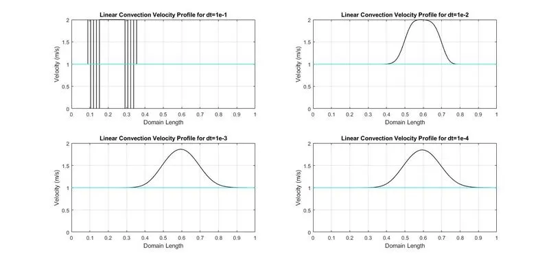
Plots comparing Initial Velocity with Final Velocity for dt=1e-1,dt=1e-2,dt=1e-3,dt=1e-4.

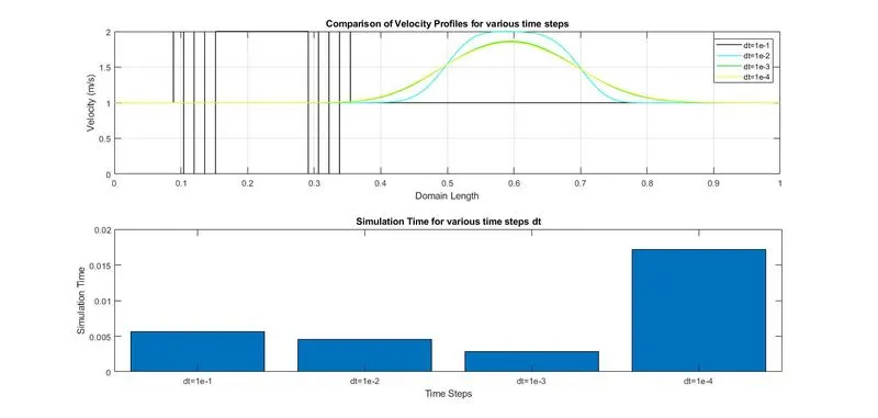
Plot comparing Final Velocity Profiles for varying time steps and Plot comparing the simulation time of velocity profiles for different time steps:

Results and Conclusion

• The velocity profile is travelling from left to right, which implies it is convecting from left to right.
• The velocity profile is stable for time steps dt=1e-2,1e-3,1e-4. The velocity profile for dt=1e-1 is filled with ripples and oscillations.
• This is because, at dt=1e-1, the solution becomes unstable and "blows up" due to the large value of time step.
• The unstability in the solution and solution blowing up is called as GIBBS PHENOMENON
• Among the 4 profiles, the velocity profile for dt=1e-2 matches perfectly with the initial velocity. The peak velocities remain the same.
• For dt=1e-3 and 1e-4, the velocity profiles remain relatively same, but the peak velocity value drops down.
• This drop in peak is due to ARTIFICIAL DIFFUSION
• Artificial diffusion is caused due to the error terms in the first order approximation of the time and space derivatives.
• These error terms are of the second order ( h(2) ) and are similar in nature to the diffusion terms in the Navier-Stokes Equations. These second order terms are neglected in the Taylor's series first order approximation of the derivatives, which leads to the diffusion of the profile and the velocity drop.
• From the bar graph comparing the simulation time for various time steps, we can see that the highest simulation time is taken for dt = 1e-4, whereas the lowest simulation time is taken for dt = 1e