To Study about the PID Controllers.

AIM : To Study about the PID Controllers.

OBJECTIVES :

1. In which situations feedforward control of DC motor fails ? Prepare a MATLAB script for feedforward control and test it.

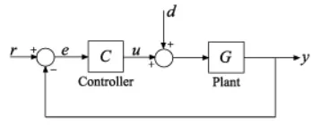
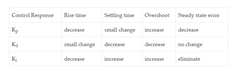
2. Assume a plant and controller. Using MATLAB PID controller block verify system response with General Observation for PID gain :

   

3. Consider below system -

   

   Use MATLAB PID tuner and prepare a table showing PID values with response time and transient behaviour coefficient.

STUDY - 1 :

Feed Forward (Control) :

• A feed forward, sometimes written feedforward, is an element or pathway within a control system that passes a controlling signal from a source in its external environment to a load elsewhere in its external environment. This is often a command signal from an external operator.

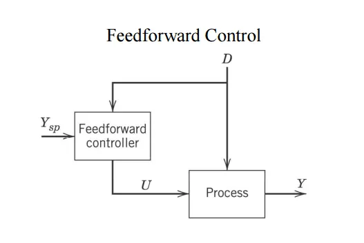
• A control system which has only feed-forward behavior responds to its control signal in a pre-defined way without responding to how the load reacts.
• it is in contrast with a system that also has feedback, which adjusts the input to take account of how it affects the load, and how the load itself may vary unpredictably. the load is considered to belong to the external environment of the system.
• In a feed-forward system, the control variable adjustment is not error-based. Instead it is based on knowledge about the process in the form of a mathematical model of the process and knowledge about, or measurements of, the process disturbances.

Situations where Feedforward Control of a DC Motor fails –

• Correct mathematical model should be known for exact disturbance rejection.

• Feedforward controller structure will change with disturbance type & sensor used.

• Recommended for slow varying process only.

• Feedforward control alone cannot give desired response hence it always has to be used with feedback controller.

• The disturbance variables must be measured on-line. In many applications, this is not feasible.

• To make effective use of feedforward control, at least an approximate process model should be available. In particular, we need to know how the controlled variable responds to changes in both the disturbance and manipulated variables. The quality of feedforward control depends on the accuracy of the process model.

• Ideal feedforward controllers that are theoretically capable of achieving perfect control may not be physically realizable. Fortunately, practical approximations of these ideal controllers often provide very effective control.

Problem Statement :

• In armature-controlled DC motors, the applied voltage Va controls the angular velocity w of the shaft.

• This example shows two DC motor control techniques for reducing the sensitivity of w to load variations (changes in the torque opposed by the motor load).

• A simplified model of the DC motor is shown above. The torque Td models load disturbances. You must minimize the speed variations induced by such disturbances.

For this example, the physical constants are :

R = 2.0;                % Ohms
L = 0.5;                % Henrys
Km = 0.1;               % torque constant
Kb = 0.1;               % back emf constant
Kf = 0.2;               % Nms
J = 0.02;               % kg.m^2/s^2
h1 = tf(Km,[L R]);            % armature
h2 = tf(1,[J Kf]);            % eqn of motion
dcm = ss(h2) * [h1 , 1];      % w = h2 * (h1*Va + Td)
dcm = feedback(dcm,Kb,1,1);   % close back emf loop
stepplot(dcm(1));

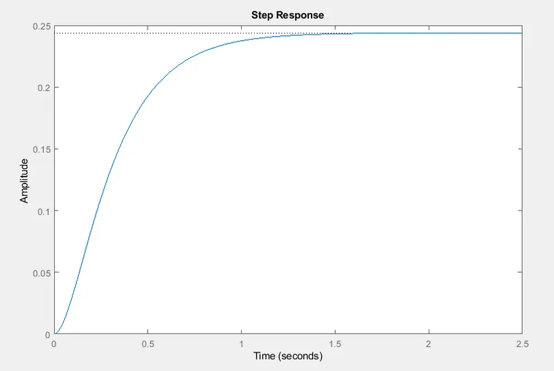
• First construct a state-space model of the DC motor with two inputs (Va,Td) and one output (w).

Feedforward DC Motor Control Design :

We can use this simple feedforward control structure to command the angular velocity w to a given value w_ref.

MATLAB Script for FeedForward Control :

R = 2.0;                % Ohms
L = 0.5;                % Henrys
Km = 0.1;               % torque constant
Kb = 0.1;               % back emf constant
Kf = 0.2;               % Nms
J = 0.02;               % kg.m^2/s^2
h1 = tf(Km,[L R]);            % armature
h2 = tf(1,[J Kf]);            % eqn of motion
dcm = ss(h2) * [h1 , 1];      % w = h2 * (h1*Va + Td)
dcm = feedback(dcm,Kb,1,1);   % close back emf loop
stepplot(dcm(1));
Kff = 1/dcgain(dcm(1))
t = 0:0.1:15;
Td = -0.1 * (t>5 & t<10);       % load disturbance
u = [ones(size(t)) ; Td];       % w_ref=1 and Td
cl_ff = dcm * diag([Kff,1]);    % add feedforward gain
cl_ff.InputName = {'w_ref','Td'};
cl_ff.OutputName = 'w';
h = lsimplot(cl_ff,u,t);
title('Setpoint tracking and disturbance rejection')
legend('cl_ff')
% Annotate plot
line([5,5],[.2,.3]);
line([10,10],[.2,.3]);
text(7.5,.25,{'disturbance','T_d = -0.1Nm'},...
            'vertic','middle','horiz','center','color','r');

The feedforward gain Kff should be set to the reciprocal of the DC gain from Va to w.

Kff =

    4.1000

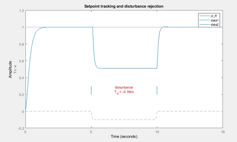
To evaluate the feedforward design in the face of load disturbances, simulate the response to a step command w_ref=1 with a disturbance Td = -0.1Nm between t=5 and t=10 seconds:

Output Plot of FeedForward Control :

• Clearly feedforward control handles load disturbances poorly.

STUDY - 2 :

Proportional Integral Derivative (PID) :

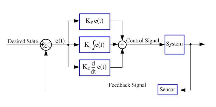
• A Proportional–Integral–Derivative controller (PID controller or three-term controller) is a control loop mechanism employing feedback that is widely used in industrial control systems and a variety of other applications requiring continuously modulated control.

• A PID controller continuously calculates an error value e(t) as the difference between a desired setpoint (SP) and a measured process variable (PV) and applies a correction based on proportional, integral, and derivative terms (denoted P, I, and D respectively).

Proportional Plot KP :

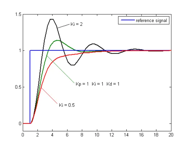
• The proportional term, K_p , is entirely based on the error and that, let's say, double the error would mean doubling K_p (applying proportional force). This therefore implies that increasing K_p is a result of the system heading in the wrong direction so K_p is increased to ensure the system goes on the right direction or at least tries to reduce the error as time passes so an increase in K_p would affect the system in such a way to adjust the heading of the system so it stays on the right path.

Integral Plot Ki :

• The derivative term, K_d , is based on the rate of change of the error so an increase in K_d implies that the rate of change of error has increased over time so double the error would result in double the force. An increase by double the change in the system's heading would take place if the system's heading is doubled in error from the previous feedback result. K_d causes the system to react faster as the error increases.

Derivative Plot Kd :

• An increase in the integral term, K_i , means that the error is increased over time. The integral accounts for the sum of error over time. Even a small increase in the error would increase the integral so the system would have to head in the right direction for an equal amount of time for the integral to balance to zero.

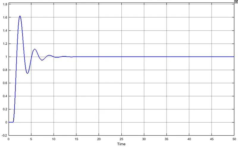
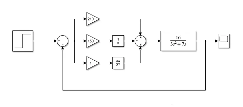
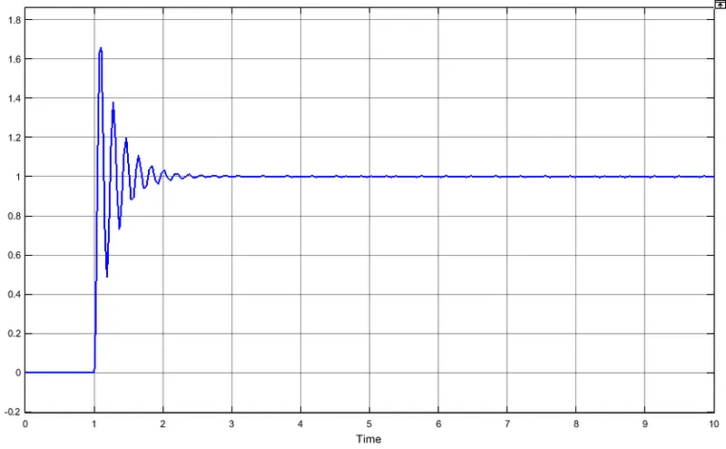
Using MATLAB PID controller block verify system response with General Observation for PID gain :

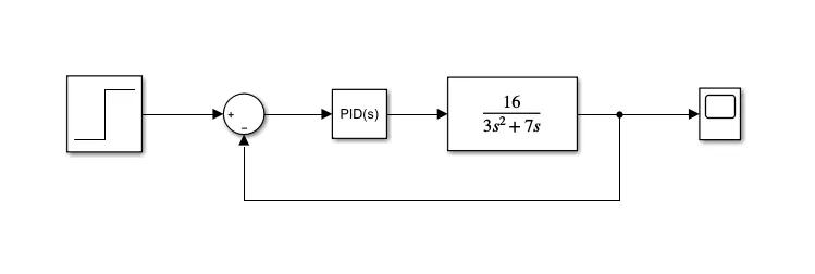
Assume a plant and controller :

Plant, G(s) = 16 / (3s³ + 7s)

Simulink Model Using PID controller block :

Output Plot :

Simulink Model Using Gain blocks :

Output Plot :

STUDY - 3 :

MATLAB PID tuner and prepare a table showing PID values with response time and transient behaviour coefficient :

Consider below system -

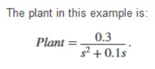
The Plant in this example is :

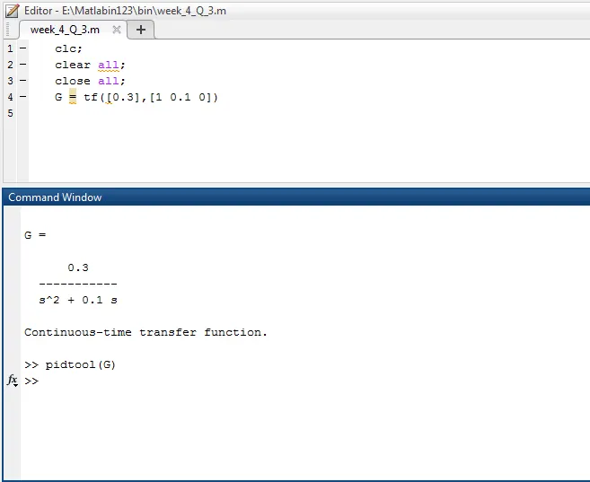
Plant, G(s) = 0.3 / (s² + 0.1s)

MATLAB Command for PID Tuner :

PID Tuner Plot Using MATLAB :

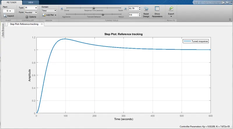
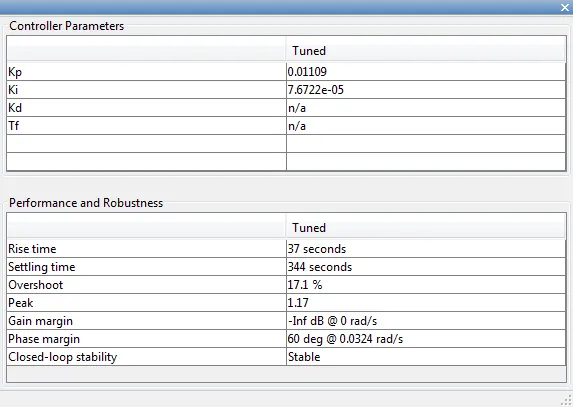
• MATLAB provides tools for automatically choosing optimal PID gains which makes the trial and error process described above unnecessary. You can access the tuning algorithm directly using pidtune or through a nice graphical user interface (GUI) using pidTuner.
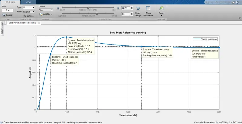
• The MATLAB automated tuning algorithm chooses PID gains to balance performance (response time, bandwidth) and robustness (stability margins). By default, the algorithm designs for a 60-degree phase margin.

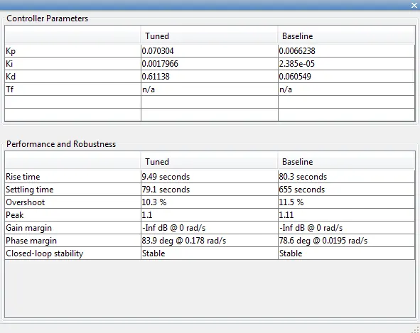
Controller Parameters Window :

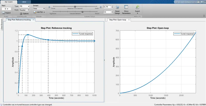
Output Plot with Controller Parameters :

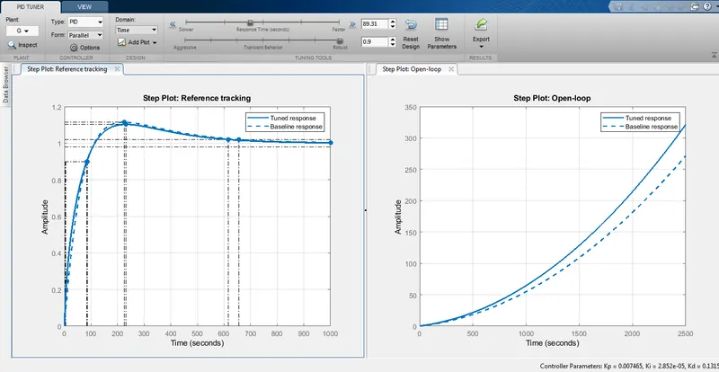
Controller Parameters Window with Baseline :

Output Plot with Open-loop Configuration :

Output Plot with Baseline Response :

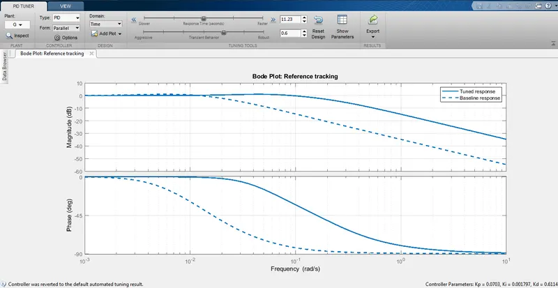
Output Bode Plot :

https://instrumentationtools.com/feedforward-vs-feedback-control/