To calculate the futuristic values of a curve by using the perfect fit, best fit and cubic fit
AIM:- To calculate the futuristic values of a curve by using the perfect fit, best fit and cubic fit.
THEORY:- Curve matching is used to calculate the future value of experiments or simulations (existing data). Depending on previous results, this can save time and cost of simulation or testing.
1.R_square(R2):-
This is the amount used to measure how well your fitted curve (predicted values) are. Another name for r_square is the square of the multiple correction coefficient and the coefficient of multiple resolution. The value of R_square varies from 0 to 1, and this value defines how accurate your curve is. The Max R-square value is very correct, and the minimum R-square value is poorly matched.
2.SSE(sum of squares of error):-
sum of squares of error is factor which is used to calculate the error of the curve. it has to be very less if possible sse has to be 0 then out predict future values would be accurate without any error.
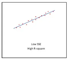
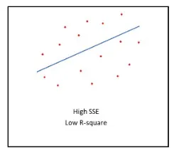
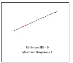
CALCULATION:-
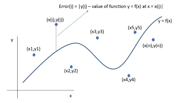
SSE(sum of squares of error) = ∑(Y(i)−f(x(i)))2
Y(i)=existing Y value with respect to x
f(x(i))=predicted Y value with respect to x
R2=(SSR)/(SST)
SSR= sum of squares of regression = ∑[f(x(i))−mean]2
SST=sum of squares of total.=SSR+SSE
PROGRAM FOR CALCULATING THE SINGLE ORDER POLYNOIMIAL PREDICTED VALUES
clear allclose all
clc
%Preparing the data
cp_data = load('data');
temperature = cp_data(:,1);
cp = cp_data(:,2);
%Applying polyfit function
co_effs = polyfit(temperature,cp,1);
predicted_cp =
polyval(co_effs,temperature);
%Calculation of futurestic values
of futurestic values
future =
polyval(co_effs,[1700:2000]);
%Plot
plot(temperature,cp,'linewidth',1,'color','r')
xlabel('temperature')
ylabel('cp')
hold on
plot(temperature,predicted_cp,'linewidth',1,'color','b')
legend('experimental value'
value','predicted value')
for i=1:length(cp);
se(i)=(predicted_cp(i)-cp(i))^2;
sr(i)=(predicted_cp(i)-mean(cp))^2;
end
%Calculation of error
SSE=sum(se');
SSR=sum(sr');
R_square=(SSR/(SSE+SSR));
RMSE=(SSE/length(temperature))^0.5;
Result:
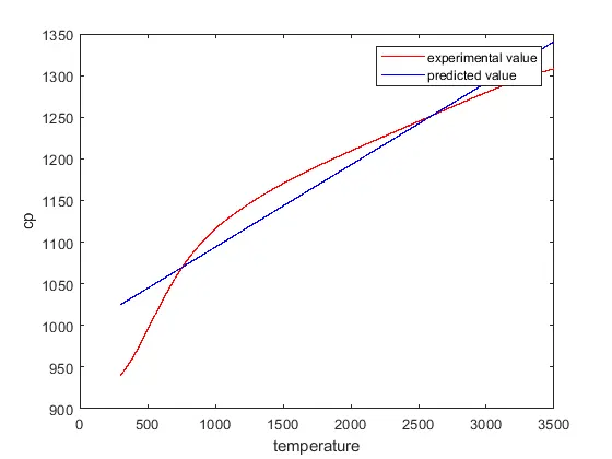
CHECKING THE RESULTS USING cftool in MATLB
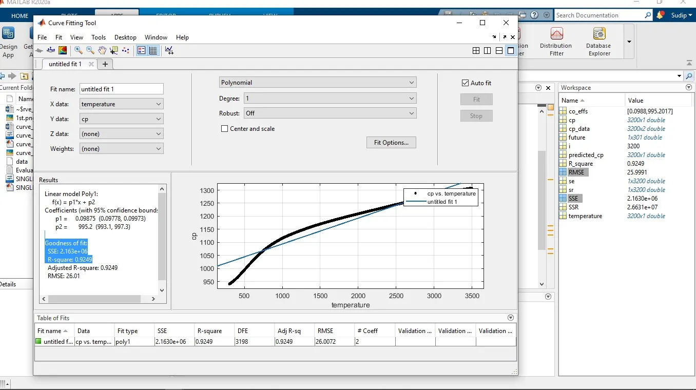
above figure shows, program for SSE and R2 is correct.
CASE1:-CURVE FIT PERFECTLY
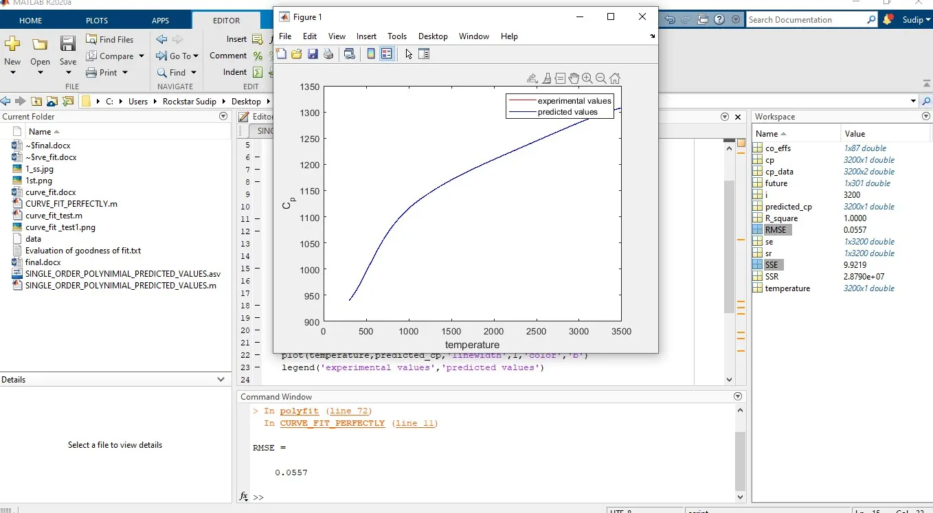
The definition curve of the correct fit should go to each point, and the sum of the squares of the error must be 0 and R2 should be 1.
In order to satisfy the above condition, the polynomial degree is approximated by increasing the polynomial degree SSE, the maximum polynomial degree value that Matlab can support is increased to 86, and the polynomial degree in the above program is multiplied by 86.
Code:
clear all
close all
clc

%preparing data.
cp_data=load('data');
temperature=cp_data(:,1);
cp=cp_data(:,2);

%applying polyfit function.
co_effs=polyfit(temperature,cp,86);
predicted_cp=polyval(co_effs,temperature);

%calculation of futurestic
values.
future =
polyval(co_effs,[1700:2000]);

%plot
plot(temperature,cp,'linewidth',1,'color','r')
xlabel('temperature')
ylabel('C_p')
hold on
plot(temperature,predicted_cp,'linewidth',1,'color','b')
legend('experimental
values','predicted values')

for i=1:length(cp);
    se(i)=(predicted_cp(i)-cp(i))^2;
    sr(i)=(predicted_cp(i)-mean(cp))^2;
end
%calculation of error
SSE=sum(se');
SSR=sum(sr');
R_square=(SSR/(SSE+SSR));
RMSE=(SSE/length(temperature))^0.5
Results are shown in below.R2=1 and SSE= 9.921
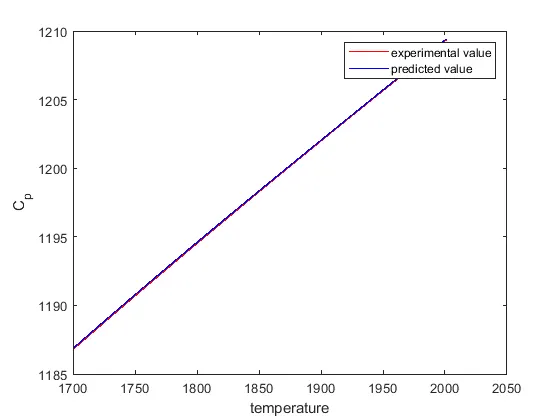
From the DATA file I have considered 1701 values, from 1701 to 2000 values I have predicted by using above equation
Code:
                                                 %loading
original data
Origional=load('data');
orig=Origional(:,2);
ori=orig(1400:1700);
B=1700+1:1700+301;

%plot the comparision
plot(B,ori,'color','r','linewidth',1)
hold on
plot(B,future,'color','b','linewidth',1)
xlabel('temperature')
ylabel('C_p')
legend('experimental
value','predicted value')

                             %program for
calculating the SSE and R_square
for i=1:length(ori);
    se(i)=(future(i)-ori(i))^2;
    sr(i)=(future(i)-mean(ori))^2;
end
SE=se.';
SR=sr.';
SSE=sum(SE);
SSR=sum(SR);
R_square=(SSR/(SSE+SSR));
Result:
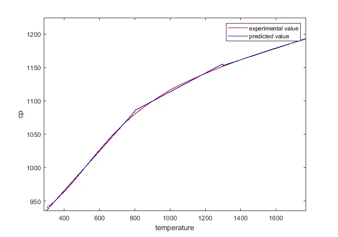
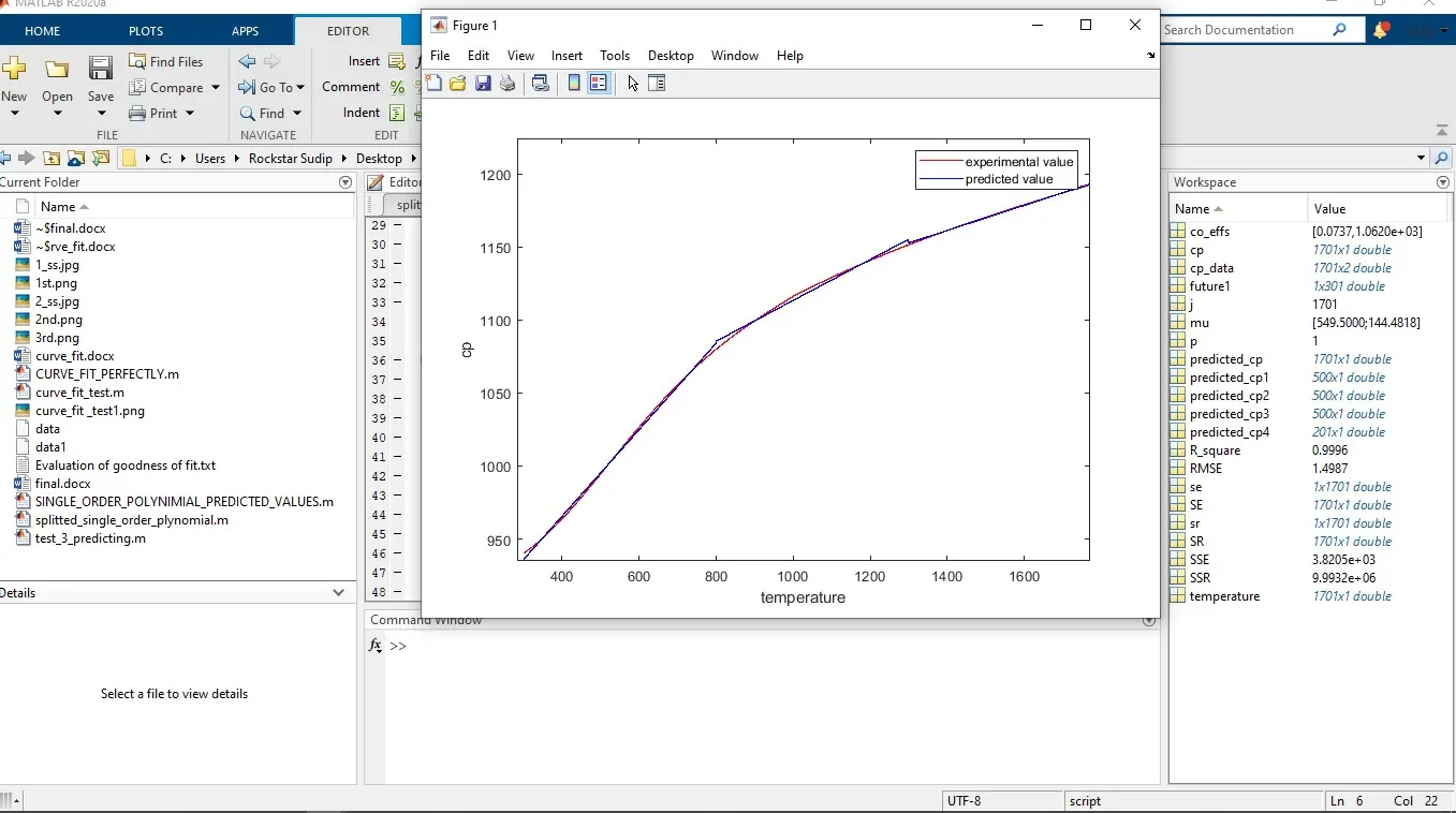
2.CURVE BEST FIT:
Best curve fit meaning which could satisfy the raw data and sum of square of error should be less and R2
I have splitted data in 4 splits with single polynomial order.
program for splitted single order plynomial.
clear all
close all
clc


     %preparing
data
cp_data = load('data1');
temperature = cp_data(:,1);
cp = cp_data(:,2);

                                     %split the
data for reducing the error
p=1;
[co_effs,~,mu] =
polyfit(temperature(1:500),cp(1:500),p);
predicted_cp1 =
polyval(co_effs,temperature(1:500),[],mu);
co_effs =
polyfit(temperature(501:1000),cp(501:1000),p);

predicted_cp2 =
polyval(co_effs,temperature(501:1000));
co_effs =
polyfit(temperature(1001:1500),cp(1001:1500),p);

predicted_cp3 = polyval(co_effs,temperature(1001:1500));
co_effs =
polyfit(temperature(1501:1701),cp(1501:1701),p);

predicted_cp4 =
polyval(co_effs,temperature(1501:1701));

predicted_cp = [predicted_cp1
;predicted_cp2 ;predicted_cp3 ;predicted_cp4];

                                                      %plot the the
results
plot(temperature,cp,'linewidth',1,'color','r')
xlabel('temperature')
ylabel('cp')
hold on
plot(temperature,predicted_cp,'linewidth',1,'color','b')
legend('raw','poly')
future1 = polyval(co_effs,[1700:2000]);

                                 %code for
calculating the R-square and SSE
for j=1:length(cp)
    se(j)=(predicted_cp(j)-cp(j))^2;
    sr(j)=(predicted_cp(j)-mean(cp))^2;
end
SE=se';
SR=sr';
SSE=sum(SE);
SSR=sum(SR);
R_square=(SSR/(SSE+SSR));
plot(temperature,cp,'linewidth',1,'color','r')
xlabel('temperature')
ylabel('cp')
hold on
plot(temperature,predicted_cp,'linewidth',1,'color','b')
legend('experimental
value','predicted value')
RMSE=(SSE/length(temperature))^0.5;
CASE3:-CUBIC FIT
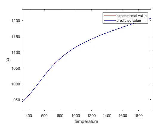
The cubic fit is the polynomial equation with 3 degrees. The cube fit of the raw data is compared and plotted in the figure below. We can reduce the SSE by dividing the data.
Code:
clear all
close all
clc


%preparing data
cp_data = load('data1');
temperature = cp_data(:,1);
cp = cp_data(:,2);

                                     %split the
data for reducing the error
p=3;
[co_effs,~,mu] =
polyfit(temperature(1:500),cp(1:500),p);
predicted_cp1 =
polyval(co_effs,temperature(1:500),[],mu);
co_effs =
polyfit(temperature(501:1000),cp(501:1000),p);

predicted_cp2 =
polyval(co_effs,temperature(501:1000));
co_effs =
polyfit(temperature(1001:1500),cp(1001:1500),p);

predicted_cp3 =
polyval(co_effs,temperature(1001:1500));
co_effs =
polyfit(temperature(1501:1701),cp(1501:1701),p);

predicted_cp4 =
polyval(co_effs,temperature(1501:1701));

predicted_cp = [predicted_cp1
;predicted_cp2 ;predicted_cp3 ;predicted_cp4];


%plot the the results
plot(temperature,cp,'linewidth',1,'color','r')
xlabel('temperature')
ylabel('cp')
hold on
plot(temperature,predicted_cp,'linewidth',1,'color','b')
legend('raw','poly')
future1 =
polyval(co_effs,[1700:2000]);

                                 %code for
calculating the R-square and SSE
for j=1:length(cp)
    se(j)=(predicted_cp(j)-cp(j))^2;
    sr(j)=(predicted_cp(j)-mean(cp))^2;
end
SE=se';
SR=sr';
SSE=sum(SE);
SSR=sum(SR);
R_square=(SSR/(SSE+SSR));
plot(temperature,cp,'linewidth',1,'color','r')
xlabel('temperature')
ylabel('cp')
hold on
plot(temperature,predicted_cp,'linewidth',1,'color','b')
legend('experimental
value','predicted value')
RMSE=(SSE/length(temperature))^0.5;
Result:
ERRORS:-
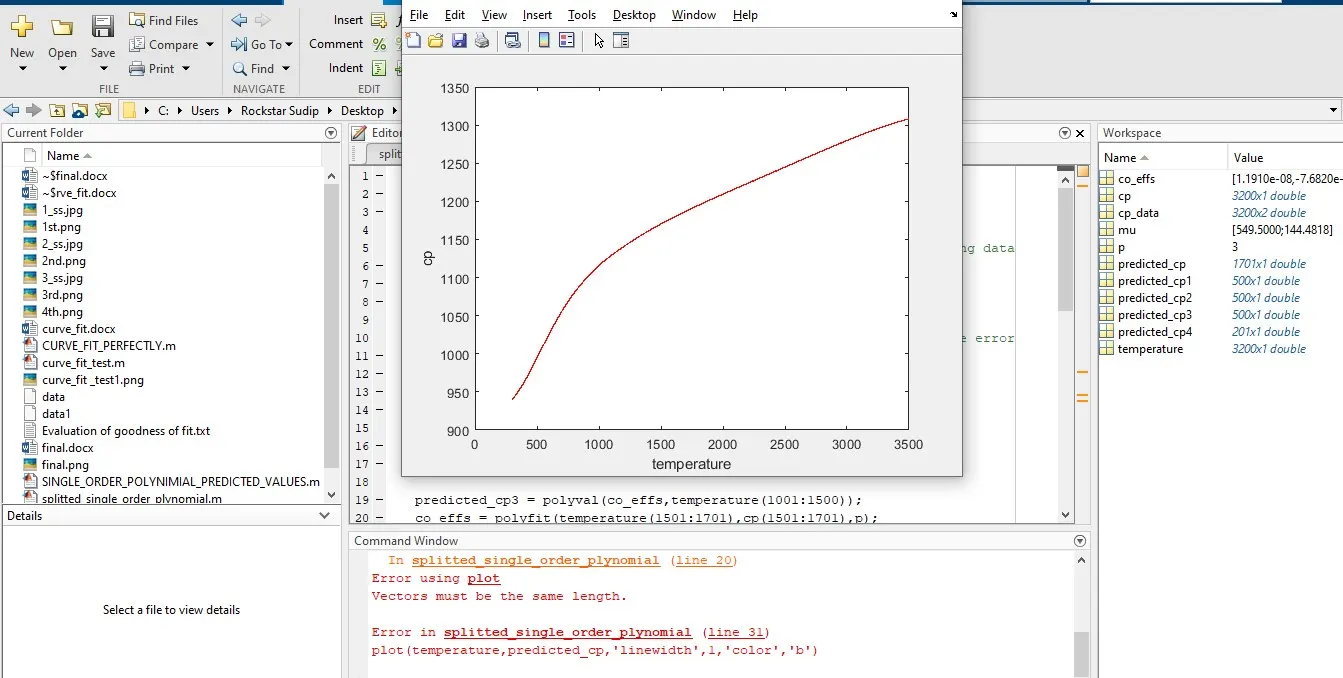
STEPS FALLOWED TO SOLVE THE ERRORS:-
1.check in google.
2.search in youtube.
3.took help from support team.
REFERENCES:-
1. https://projects.skill-lync.com/projects/Curve-Fitting-and-criterion-to-choose-best-fit-41860
2.MATLAB support book.