THERMODYNAMIC RANKINE CYCLE

AIM:

To write a code to simulate Rankine Cycle and to determine the state points.

OBJECTIVE:

• To calculate the state points of the Rankine Cycle based on user inputs.
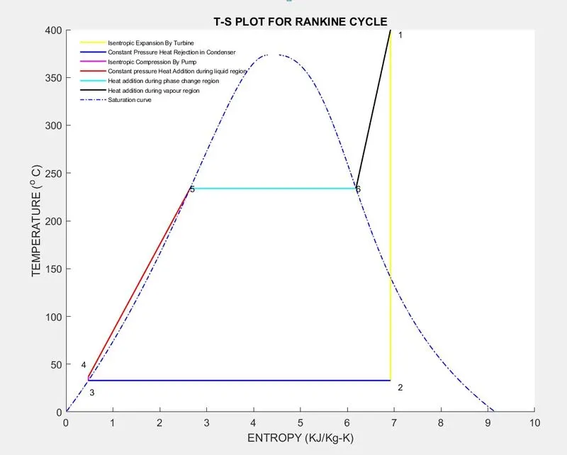
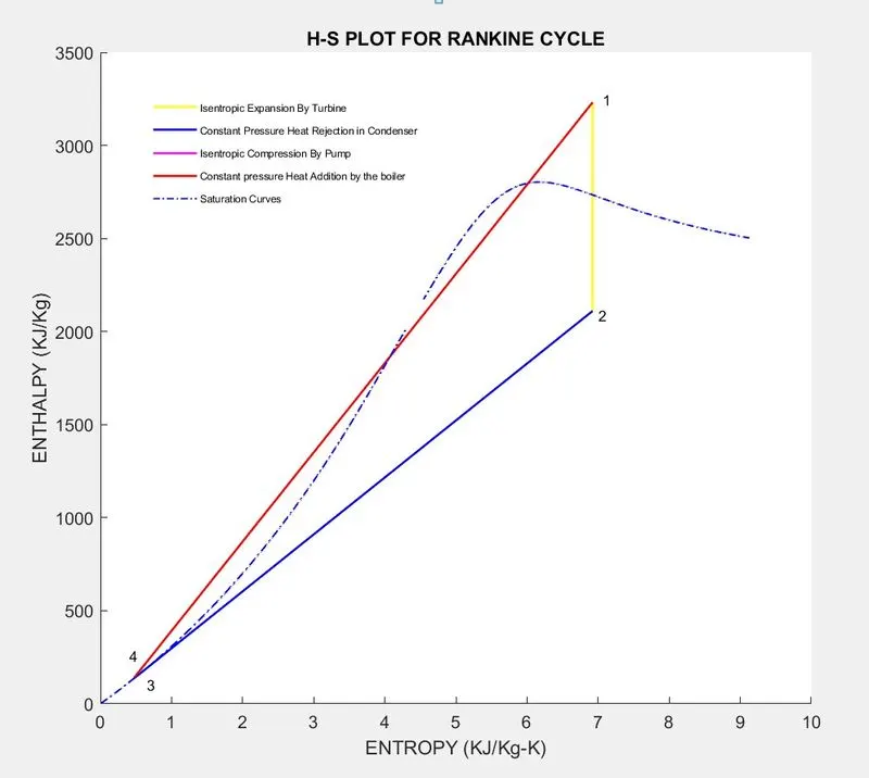
• Plot the corresponding T-s and h-s plots for the given set of inputs.
• To explain the working of a rankine cycle
• By using, standard Xsteam library to get the steam table data for water, to calculate the points in between the state variables.
• To calculate Net workdone and Back Work Ratio of rankine cycle

INTRODUCTION:

RANKINE CYCLE:

The Rankine cycle is an idealized thermodynamic cycle describing the process by which certain heat engines such as steam turbines or reciprocating steam engines, allow mechanical work to be extracted from a fluid as it moves between a heat source and a heat sink. Rankine engines generally operate in a closed loop where the working fluid is reused.

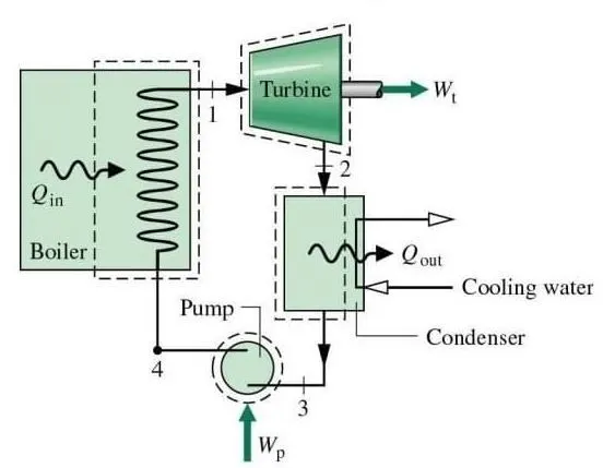
PROCESS IN RANKINE CYCLE:

PROCESS (1-2): Isentropic Expansion By the Turbine:

The high Pressure and Temperature of a steam enters into the turbine area, where it expands. As the steam expands, it strikes with the turbine blades, which convert the thermal energy of the steam into rotational energy (mechanical work) (ie;) work done by the Turbine (Wt). As the turbine blades are rotated, they also rotate a crankshaft that further rotates the coil of the generator. As the coil rotates in a magnetic field, it produces electricity. During this whole process, the pressure and temperature of the steam decrease.

PROCESS (2-3): Constant pressure heat rejection in a Condenser:

After the expansion process, the vapour or steam enters into the Condenser . In this condensation process, the vapour is condensed to convert it into saturated liquid. During this process, the vapour rejects heat (Q_out), but its liquid pressure remains the same.

PROCESS (3-4): Isentropic Compression By the Pump:

In this stage, a Pump uses to transfer the saturated liquid or other working medium from the water body (canal or tank) into the boiler. The pump requires a small amount of energy for initial pumping. It pumps the fluid by increasing the pressure of the fluid, but fluid entropy remains the same. For initial pumping, the work done on the pump is required (ie;) Wp.

PROCESS (4-1): Constant pressure heat addition By the Boiler:

As the water is delivered into the boiler by feed water pump, an external heat source (Coal or lignite) provides heat to the boiler (Q_in). The boiler heated the water at constant pressure and converts it into dry saturated vapour (steam). During this process, the enthalpy of the liquid changes, and pressure remains constant.

SATURATED LIQUID & VAPOUR:

The temperature of water changes with ambient pressure, such that a low pressure corresponds to a low boiling point temperature and a high pressure increases the boiling point temperature.

When a saturation condition is reached, the liquid phase and the vapor phase are in equilibrium with one another, i.e., both phases can exist simultaneously.

If a small amount of energy is added to saturated liquid, it turns into vapor at constant temperature. A liquid that is about to vaporize is called a saturated liquid. Likewise, if a small amount of energy is removed from saturated vapor, it will condense to liquid at constant temperature. A vapor that is about to condense is called a saturated vapor.

XSTEAM LIBRARY:

XSteam is a separate library for Matlab that contains, different properties of water and water vapor. XSteam works as a function that call exactly the state variables and as plot or polyphytic.

DRYNESS FRACTION:

Dryness fraction of steam (x) is the Ratio of mass of dry steam to the summation of the mass of dry steam and mass of water vapour in the mixture.

GOVERNING EQUATIONS OF RANKINE CYCLE:

1. Workdone By the Turbine (W_t) = (h1-h2)

The work done by the turbine is calculated by neglacting Surrounding heat transfer, Kinetic energy and potential energy.

2. Constant pressure heat rejection by the condenser (q_out) = (h2-h3)
3. Workdone By the Pump (W_p) = (h4-h3)
4. Constant pressure heat addition by the Boiler (q_in) = (h1-h4)
5. Net workdone (N_w) = (workdone by pump - workdone by turbine) = (W_t -W_p)
6. Thermal Efficiency (T_effi) = (Net workdone/Heat addition) = (N_w/q_in)
7. Back Work Ratio (BWR) = (Pump work input/Turbine work Output) = (W_p/W_t)
8. Dryness fraction (x) = mass of dry steam /mass of dry steam and mass of water vapour in the mixture

NOTATIONS USED:

h1,h2,h2,h4,h5,h6 - Specific Enthalpy's at state points

s1,s2,s3,s4,s5,s6 - Specific Entropy's at state points

t1,t2,t3,t4,t5,t6 - Specific Temperature at state points

p1,p2,p3,p4 - Specific pressure at state points

Tsat_p - Saturation Temperature

hV_p - Saturated Vapour Enthalpy as a function of pressure

hL-p - Saturated Liquid Enthalpy as a function of pressure

h_ps - Enthalpy as a function of pressure and Entropy

sV_p - Saturated vapour entropy as a function of pressure

sL_p - Saturated liquid entropy as a function of pressure

sV_T - Saturated vapour entropy as a function of Temperature

sL_T - Saturated liquid entropy as a function of Temperature

hV_T - Saturated vapour enthalpy as a function of Temperature

hL_T - Saturated liquid enthalpy as a function of Temperature

s_pT - Specific entropy as a function of pressure and temperature (Returns saturated vapour entalpy if mixture.)

Cp_ps - Specific isobaric heat capacity as a function of pressure and entropy.

Cv_ps - Specific isochoric heat capacity as a function of pressure and entropy.

STEPS INVOLVED IN CODING:

STEP 1: Assigning the process of Rankine cycle

STEP 2: Assigning the input parameters from the user

STEP 3: Determining the thermodynamic state conditions

STEP 4: Using, XSteam library, different properties of water and water vapor are determined

STEP 5: Determining the enthapy(h), entropy(s) and temperature (t) of liquid and vapour region

STEP 6: Evaluating net workdone of rankine cycle

STEP 7: Evaluating Back Work Ratio and efficiency of rankine cycle

STEP 8: Creating the saturation curve by defining the for loop for the temperature range to draw

STEP 9: Inside the for loop, defining the enthalpy and entropy as a function of temperature

STEP 10: Plotting T-S and H-S diagram of rankine cycle

STEP 11: The assigned input of state conditions and state variables are executed in the command window

CODING:

%Rankine cylce Simulate
%To find the state points of the process, Thermal efficiency of rankine cycle, Back work ratio
clear all
close all
clc
%To be print in the Window screen

fprintf('                      RANKINE CYCLE SIMULATOR                 n')
fprintf('Process (1-2): Isentropic Expansion In the Turbinen')
fprintf('Process (2-3): Constant Pressure Heat Rejection by the Condensern')
fprintf('Process (3-4): Isentropic Compression In the Pumpn')
fprintf('Process (4-1): Constant Pressure Heat Addition by the Boilern')

%Inputing from the user
p1=input('Enter the inlet pressure at the turbine (in Bars):');
t1=input('Enter the inlet temperature at the turbine (in deg Celcius):');
p2=input('Enter the Inlet Pressure at the Condenser (in Bars):');

%Determining the Thermodynamic state conditions
%Dtermining of state points -1 (P1,T1,H1,S1): (Inlet to Turbine)
%P1 & T1 are given

h1=XSteam('h_pT',p1,t1);  %h_pT	Entalpy as a function of pressure and temperature
s1=XSteam('s_pT',p1,t1);  %s_pT	Specific entropy as a function of pressure and temperature (Returns saturated vapour entalpy if mixture.)

%Dtermining of state points -2 (P2,T2,H2,S2): (Inlet to Condenser)
%P2 is given
s2=s1;  %Specific entropy is constant for adiabatic Reversible process

%Determining saturated entropy's State
sl2=XSteam('sL_p',p2); %saturated liquid entropy
sv2=XSteam('sV_p',p2); %Saturated vapour entropy
%Determining saturated enthalpy's State
hl2=XSteam('hL_p',p2); %Saturated liquid enthalpy
hv2=XSteam('hV_p',p2); %Saturated vapour enthalpy
%Determining the dryness fraction @ state point 2
x2=(s2-sl2)/(sv2-sl2);

h2=hl2+(x2*(hv2-hl2)); %Mixture of liquid and vapour enthalpy.

%Determination of state points -3 (P3,T3,H3,S3): (Inlet to Pump)

p3=p2; %Pressure is constant @ state 2 and 3
%Determining the saturated temperature
t3=XSteam('Tsat_p',p3);
t2=t3; %Temperature is contant @state 2 and 3
h3=XSteam('hL_p',p3); %Saturated liquid enthalpy as a function of pressure
s3=XSteam('sL_p',p3); %Saturated liquid entropy as a function of pressure

%Dtermination of state points -4 (P4,T4,H4,S4): (Inlet to the Boiler)
s4=s3; %Entropy remains contant at state
p4=p1; %At constant pressure heat addition, pressure remains constant
h4=XSteam('h_ps',p4,s4); %Specific enthalpy as a function of pressure and entropy

%Calculating temperature >> Using (t3/t4)=(p3/p4)^gamma

cp4=XSteam('cp_ps',p4,s4);  %Cp_ps	Specific isobaric heat capacity as a function of pressure and entropy.
cv4=XSteam('cv_ps',p4,s4);  %Cv_ps	Specific isochoric heat capacity as a function of pressure and entropy.
n=cp4/cv4;
gamma=(n-1)/n;
t4=(t3)/(p3/p4)^gamma; %Temperature at state point 4

%Determination of Temperature, enthalpy and entropy at liquid and vapour region
%At Liquid region
s5=XSteam('sL_p',p1);  %Specific entropy at liquid region
h5=XSteam('hL_p',p1);  %Specific enthalpy at liquid region

%At vapour region
s6=XSteam('sV_P',p1);  %Specific entropy at vapour region
h6=XSteam('hV_p',p1);  %Specific enthalpy at vapour region

%Temperature at liquid and vapour region is constant
t6=XSteam('Tsat_p',p1);
t5=t6;   % Temperature are constant

%STATSTICAL ANALYSIS OF RANKINE CYCLE

%calculation for turbine work
W_t=(h1-h2);

%Calulation of pump work
w_p=(h4-h3);

%Calculation of net work
N_w=(W_t-w_p);

%Calulating heat addition
q_in=(h1-h4);

%Calulating heat Rejection
q_out=(h2-h3);

%Calculating thermal efficiency

T_effi=(N_w/q_in)*100;

%Calculating specific steam consumption
ssc=3600/N_w;

%Calculating Back Work Ratio
BWR=w_p/W_t;


%SATURATION CURVE
%Using for loop for saturation curve (Enthalpy and Entropy @ liquid and vapout state's)
T=linspace(1,t1,1000); %Temperature range with 1000 intervels
for i=1:length(T)
  %Enthalpy at liquid and vapour state 
  h_l(i)=XSteam('hL_T',T(i)); %Saturated Enthalpy
  h_v(i)=XSteam('hV_T',T(i)); %Saturated Enthalpy
  %Entropy at liquid and vapour state 
  s_l(i)=XSteam('sL_T',T(i)); %Saturated Entropy
  s_v(i)=XSteam('sV_T',T(i)); %Saturated Entropy
end

%PLOTTING T-S AND H-S DIAGRAM FOR RANKINE CYCLE

%Plotting of T-S diagram
figure(1) %Creates separate window for plot 1
hold on
text(s1,t1,'1'); %Add text in the state point 1
plot([s1 s2],[t1 t2],'color','y','linewidth',1.5);
text(s2,t2,'2'); %Add text in the state point 2
plot([s2 s3],[t2 t3],'color','b','linewidth',1.5);
text(s3,t3,'3'); %Add text in the state point 3
plot([s3 s4],[t3 t4],'color','m','linewidth',1.5);
text(s4,t4,'4'); %Add text in the state point 4
plot([s4 s5],[t4 t5],'color','r','linewidth',1.5);
text(s5,t5,'5'); %Add text in the state point 5
plot([s5 s6],[t5 t6],'color','c','linewidth',1.5);
text(s6,t6,'6'); %Add text in the state point 6
plot([s6 s1],[t6 t1],'color','k','linewidth',1.5);

%Sturation curve draw
plot(s_l,T,'color','b','linestyle','-.','linewidth',1);
plot(s_v,T,'color','b','linestyle','-.','linewidth',1);
xlabel('ENTROPY (KJ/Kg-K)'); %Labelling x axes
ylabel('TEMPERATURE (^o C)');%Labelling y axis
title('T-S PLOT FOR RANKINE CYCLE')
legend('Isentropic Expansion By Turbine','Constant Pressure Heat Rejection in Condenser','Isentropic Compression By Pump','Constant pressure Heat Addition during liquid region','Heat addition during phase change region','Heat addition during vapour region','Saturation curve','location','northwest','fontsize',7);
legend('boxoff'); %Surrounding box is hidden in legend
warning('off') %warning off 
set(gca,'fontsize',12); %seting the font size limits from axes


%Plotting (H-S diagram)
figure(2) % Creates separate window for plot 2  
hold on
text(s1,h1,'1'); %Add text in the state point 1
plot([s1 s2],[h1 h2],'color','y','linewidth',1.5);
text(s2,h2,'2'); %Add text in the state point 2
plot([s2 s3],[h2 h3],'color','b','linewidth',1.5);
text(s3,h3,'3'); %Add text in the state point 3
plot([s3 s4],[h3 h4],'color','m','linewidth',1.5);
text(s4,h4,'4'); %Add text in the state point 4
plot([s4 s1],[h4 h1],'color','r','linewidth',1.5);

%Sturation curve draw
plot(s_l,h_l,'color','b','linestyle','-.','linewidth',1);
plot(s_v,h_v,'color','b','linestyle','-.','linewidth',1);
xlabel('ENTROPY (KJ/Kg-K)'); %x labelling
ylabel('ENTHALPY (KJ/Kg)'); %y labelling
title('H-S PLOT FOR RANKINE CYCLE')
legend('Isentropic Expansion By Turbine','Constant Pressure Heat Rejection in Condenser','Isentropic Compression By Pump','Constant pressure Heat Addition by the boiler','Saturation Curves','location','northwest','fontsize',7);
legend('boxoff'); %Surrounding box is hidden in legend
warning('off') %warning off
set(gca,'fontsize',12); %seting the font size limits from axes


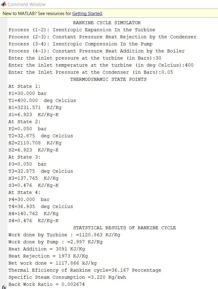
fprintf('                     THERMODYNAMIC STATE POINTS  n')

fprintf('At State 1:n')
fprintf('P1=%.3f barn',p1)
fprintf('T1=%.3f  deg Celciusn',t1)
fprintf('H1=%.3f  KJ/Kgn',h1)
fprintf('S1=%.3f  KJ/Kg-Kn',s1)

fprintf('At State 2:n')
fprintf('P2=%.3f  barn',p2)
fprintf('T2=%.3f  deg Celciusn',t2)
fprintf('H2=%.3f  KJ/Kgn',h2)
fprintf('S2=%.3f  KJ/Kg-Kn',s2)

fprintf('At State 3:n')
fprintf('P3=%.3f  barn',p3)
fprintf('T3=%.3f  deg Celciusn',t3)
fprintf('H3=%.3f  KJ/Kgn',h3)
fprintf('S3=%.3f  KJ/Kg-Kn',s3)

fprintf('At State 4:n')
fprintf('P4=%.3f  barn',p4)
fprintf('T4=%.3f  deg Celciusn',t4)
fprintf('H4=%.3f  KJ/Kgn',h4)
fprintf('S4=%.3f  KJ/Kg-Kn',s4)


fprintf('                      STATSTICAL RESULTS OF RANKINE CYCLEn')
fprintf('Work done by Turbine : =%.3f KJ/Kg n',W_t)
fprintf('Work done by Pump : =%.3f KJ/Kg n',w_p)
fprintf('Heat Addition = %3.f KJ/Kg n',q_in)
fprintf('Heat Rejection = %3.f KJ/Kgn',q_out)
fprintf('Net work done = %.3f kJ/kgn',N_w)
fprintf('Thermal Eficiency of Rankine cycle=%.3f Percentagen',T_effi)
fprintf('Specific Steam Consumption =%.3f Kg/kwh n',ssc)
fprintf('Back Work Ratio = %f n',BWR)

CODING EXPLANATION:

• Assigning the Rankine cycle process using fprintf command. By using fprintf command the conditions are executed in the command window.
• Assignin the input of pressure of inlet to turbine (p1), inlet to condenser (p2) and inlet temperature (t1), these parameters are assigned by the user by using input command.
• By using the inlet pressure and temperature the thermodynamic state conditions are determined by using XSteam library.
• h_pT Entalpy as a function of pressure and temperature by which inputting the p1 & t1 the enthalpy (h1) will be determined
• s_pT Specific entropy as a function of pressure and temperature (Returns saturated vapour entalpy if mixture) by which inputting the p1 & t1 the entropy (s1) will be determined.
• Determining the state point variables at 2, In process of condenser the entropy of states remains constant s2=s1.
• At state point 2, the saturated enthalpy and entropy of liquid and vapour states are determined as a function of pressure(p2) respectively.
• Determining the dryness fraction (x2) at state point 2 to find the enthalpy (h2)
• At state point 3, the temperature and pressure are constant p3=p2 & t3=t2
• From the condenset outlet the water is in liquid state, from which at state point 3 the enthalpy (h3) and entropy (s3) of saturated luquid are founded,
• At state point 4, the entropy (s4=s3) & pressure (p4=p1) are constant, by which the spsecific enthalpy(h4) are determined as a function of pressure and entropy.
• The temperature (t4) are determined using gas law
• Then, from the boiler the liquid are boiled as liquid region and then it's phases transfered to vapour region.
• The entroy(s5 & s6) ,enthalpy (h5,h6) & temperature (t5,t6) are determined using XSteam library.
• Evaluating the Net Workdone, Eficiency and Back Work Ratio by governing equations
• Plotting the saturation curve, the temperature ranges (T) are defined with equal intervels
• Using for loop the temperature intervels are iterated.
• Inside the for loop, the enthalpy and entropy at liquid and vapour states are determined as a function of temperature range
• Plotting Rankine cycle diagram
• Plotting T-S diagram, figure(1) is created to plot separate window for T-S diagram
• Plotting the state variables and saturation curve.
• Plotting H-S diagram, figure(2) is created to plot separate window for H-S diagram
• Plotting the state variables and saturation curve.
• Using fprintf command the state points are executed in the command window
• The, %f converts floating-point values to text using fixed-point notation by which the state point values are executed using fprintf command

PLOTTINGS OF RANKINE CYCLE:

PLOTTING OF T-S DIAGRAM:

PLOTTING OF H-S DIAGRAM:

SCREENSHOT OF COMMAND WINDOW:

ERRORS FACED WHILE PROGRAMMING:

• The XSteam was not defined properly

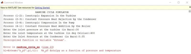
• While defining the Temperature range for saturation curve

STEPS TO OVERCOME THOSE ERRORS:

• The XSteam id properly assigned
• The temperature range is defined correctly and entropy and enthalpy for liquid and vapour region is assigned properly.

CONCLUSION:

• A code to simulate Rankine Cycle has been done and the state points of the Rankine Cycle based on user inputs are executed
• Plots corresponding T-s and h-s diagram for the given set of inputs are plotted using state point variables.
• The working of a rankine cycle simulator are explained.
• Evaluation of Net workdone,Efiiciency and Back Work Ratio of rankine cycle are determined and executed in the command window.

REFERENCE:

1. https://www.mathworks.com/matlabcentral/fileexchange/9817-x-steam-thermodynamic-properties-of-water-and-steam
2. https://www.nuclear-power.com/nuclear-engineering/thermodynamics/thermodynamic-cycles/rankine-cycle-steam-turbine-cycle/theory-of-rankine-cycle-equations-and-calculation/
3. https://www.tlv.com/global/TI/steam-theory/wet-steam-dry-steam.html
4. https://www.theengineerspost.com/rankine-cycle/