Supervised Learning - Prediction Week 3 Challenge
L1 vs L2 Regularization: The intuitive difference
A lot of people usually get confused which regularization technique is better to avoid overfitting while training a machine learning model.
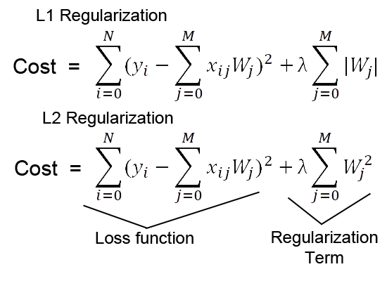
QUESTION2:The main intuitive difference between the L1 and L2 regularization is that L1 regularization tries to estimate the median of the data while the L2 regularization tries to estimate the mean of the data to avoid overfitting.
As we can see from the formula of L1 and L2 regularization, L1 regularization adds the penalty term in cost function by adding the absolute value of weight(Wj) parameters, while L2 regularization adds the squared value of weights(Wj) in the cost function.
While taking derivative of the cost function, in L1 regularization it will estimate around the median of the data. Let me explain it in this way — Suppose you take an arbitrary value from the data (assume data is spread along a horizontal line). If you then move in one direction to some distance d, suppose in the backward direction, then while calculating loss, the values to the one side (let say left side) of the chosen point will have a lesser loss value while on another side will contribute more in the loss function calculation.
Therefore, to minimize the loss function, we should try to estimate a value that should lie at the mid of the data distribution. That value will also be the median of the data distribution mathematically.
While in L2 regularization, while calculating the loss function in the gradient calculation step, the loss function tries to minimize the loss by subtracting it from the average of the data distribution.
That’s the main intuitive difference between the L1 (Lasso) and L2 (Ridge) regularization technique.
Another difference between them is that L1 regularization helps in feature selection by eliminating the features that are not important. This is helpful when the number of feature points are large in number.
That’s all from my side this time. Hope I am able to explain the intuitive difference between both the regularization techniques.
QUESTION3:
Loss Functions for Regression
Algorithms like Linear Regression, Decision Tree, Neural networks, majorly use the below functions for regression problems.
- Mean Squared Loss(Error)
- Mean Absolute Loss(Error)
- Huber Loss
Mean Squared Error
Mean squared error (MSE) can be computed by taking the actual value and predicted value as the inputs and returning the error via the below equation (mean squared error equation).

Here N is the number of training samples, yi is the actual value of the ith sample, and yi_hat is the predicted value of the corresponding sample. This Equation gives the mean of the square of the difference.
Mean Squared Error is most commonly used as it is easily differentiable and has a stable nature.
Why Mean Squared Error?
As we have seen, the equation is very simple and thus can be implemented easily as a computer program. Besides that, it is powerful enough to solve complex problems.
The equation we have is differentiable hence the optimization becomes easy. This is one of the reasons for adopting MSE widely. Let’s build intuition mathematically with an assumption that you are familiar with calculus.
The below is the general equation for the differentiation of x^n:

This implies for n=2 (squared error), the equation will be:

Comparing this standard differentiation formula to MSE with removing the normalization part (which is computing the mean) and the summation part (we can ignore the mean and summation for simplicity), the result will be:

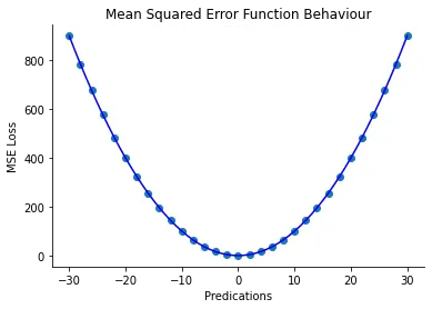
Here is what it looks like when we plot a graph of MSE loss against a signed difference between the actual value and the predicted value.
When to use MSE?
Mean Squared Error is preferred to use when there are low outliers in the data. This is one of the drawbacks of MSE.
As the MSE loss uses a square of a difference, the loss will be huge for outliers and it adversely affects the optimized solution. Using standardized data is efficient for better optimization using this loss.
Advantages
- Simple Equation, Can be optimizedg easily compared to other equations.
- Has proven its ability over the years, this is majorly used in fields like signal processing
Disadvantages
- It is highly affected by Outliers. So if the data contains outliers, better not to use it.
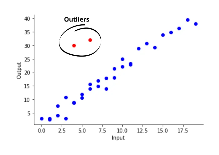
Outliers refer to the data that does not follow the same pattern(trend) as most data are following. The below graph shows a clear explanation of this:
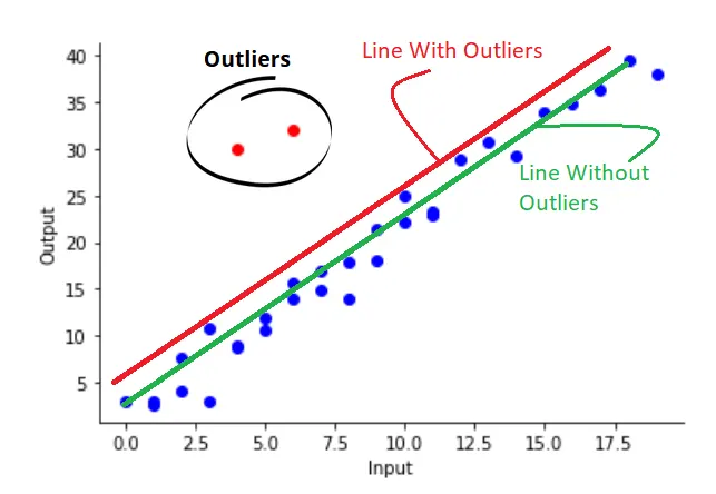
The linear regression line with MSE loss will tend to align with those outliers.
QUESTION4,
Choosing the Ideal Learning Rate
When training a model, the ‘learning rate’ is often considered to be the most important hyper-parameter. Choosing the optimal learning rate can greatly improve the training of a neural network and can prevent any odd behavior that may occur during stochastic gradient descent.
Why Is Choosing the Right Learning Rate Important?
Stochastic gradient descent (SGD) is an optimization algorithm that helps the loss function converge to the global minimum, or where the loss is at its lowest point. It behaves just like gradient descent, but also has batches to increase the computational efficiency. Gradient descent is performed to each of these smaller batches instead of the entire training set size. After each iteration of training, SGD takes one step closer to the global minimum until it has reached this point. The learning rate hyper-parameter is the step size that SGD uses to converge.
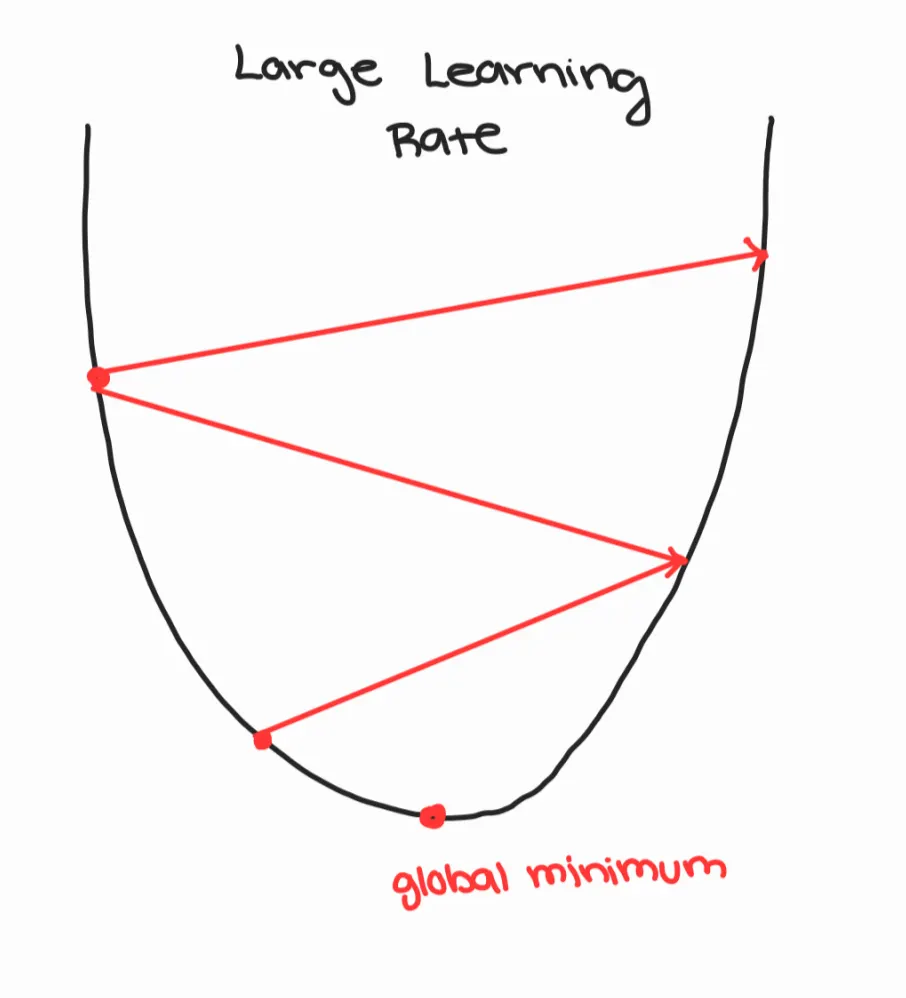
If the learning rate is too large, then SGD can overshoot and completely miss the global minimum, making the loss worse.
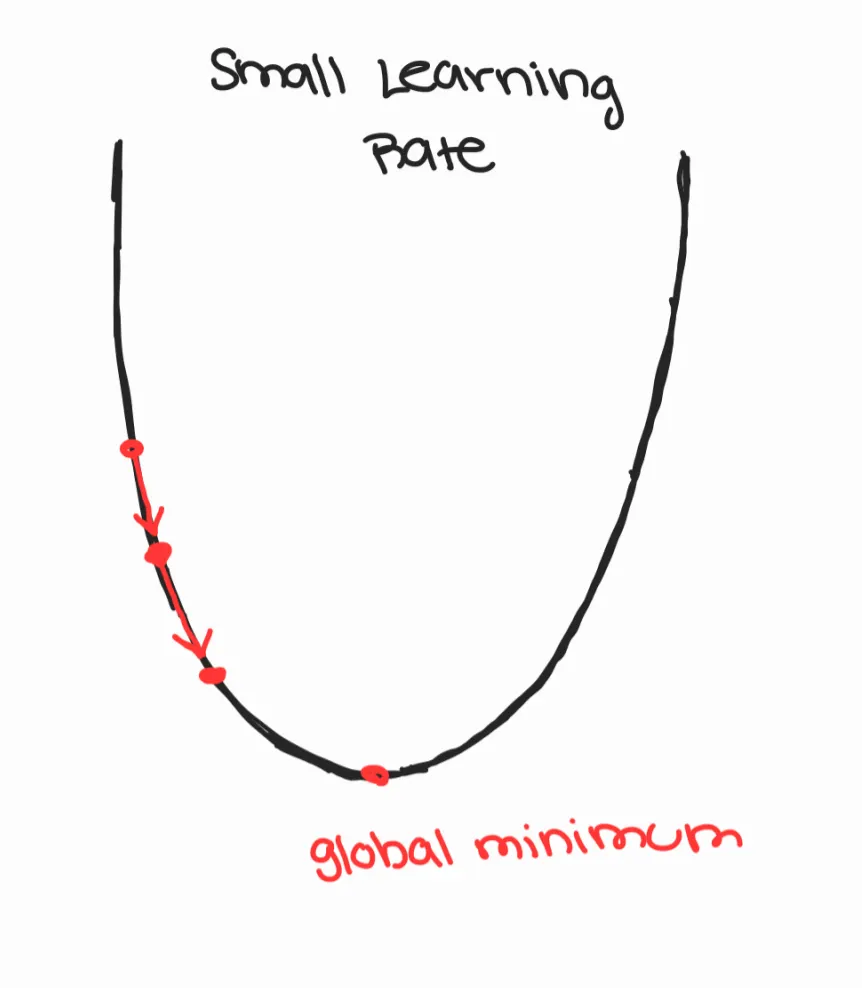
If the learning rate is too small, SGD may take a long time to converge as it will be taking small steps towards the global minimum. In cases where the function is non-convex, the model may get stuck at a local minimum.
We want to find the perfect learning rate, one that doesn’t take many iterations to converge while also eventually finding the lowest loss.
How Can We Do This?
One way to approach this problem is to try different values for the learning rate and choose the value that results in the lowest loss without taking too much time to converge. Some common values for learning rates include 0.1, 0.01, 0.001, and 0.0001. This is a guess and check method that will not be efficient and accurate all the time.
A better approach is to start with a large value for the learning rate and gradually decrease this value. Weights are initialized randomly and may be far from the optimal value. Therefore, starting with a large learning rate will be beneficial. A lower learning rate, later on, will better optimize weights closer to the optimal value by changing them only slightly. This is known as learning rate decay and is shown to help with optimization and generalization.
Cyclical Learning Rates
A paper by Leslie N. Smith, “Cyclical Learning Rates for Training Neural Networks”, discusses another method of choosing an optimal learning rate.
In this method, the learning rate is gradually increased for each mini-batch until the loss starts to explode. The learning rate versus the loss is plotted for each iteration. The paper mentions how the ideal learning rate is the point where the loss is still decreasing, right before it reaches the global minimum.
Fastai Learning Rate Finder
Fastai is a free, open-source library for deep learning. It has numerous useful and easy-to-use tools for creating and training neural networks. This library was created by Jeremy Howard and a team of data scientists who have a detailed course on how to navigate and use fastai.
Included in this library is a learning rate finder.
With two simple lines, fastai can find the ideal learning rate for the model by plotting different learning rates against the loss.
learn.lr_find()
learn.recorder.plot()
The following line of code changes the learning rate from a larger value to a smaller value throughout training.
learn.fit_one_cycle(4, lr_max=slice(1e-3,1e-4))