Unsupervised Learning - Kmeans Week 11 Challenge
QUESTION1
ANS:
Similarity Measures for Categorical Data
Part 0:Filler
Categorical data (also known as nominal data) has been studied for a long time in various contexts. However computing similarity between categorical data instances is not straightforward owing to the fact that there is no explicit notion of ordering between categorical values.To overcome this problem, several data-driven similarity measures have been proposed for categorical data. The behavior of such measures directly depends on the data.
Let us try to get to know some of the measures. To define these measures lets begin with a few notations.
Part 1: Definitions
- Consider a categorical data set D containing N data points (rows), defined over a set of d categorical attributes let Aₖ represent the kth attribute where K=1,2,3…d. Let Aₖ take nₖ unique values in the data set.
- Let fₖ(x) be the frequency of the attribute Aₖ taking the value x which is one of the nₖ values.
- let pₖ(x) be the sample probability of the attribute Aₖ taking the value x.
There are many similarity measures in the literature here we are only going to define a few of them and implement them in python.
What is the relationship between similarity measure and distance measure?
- sim = ¹⁄₁₊ₗₑₙ where sim = similarity and len= distance.
Similarity measures assigns value between two data instances X and Y belonging to the data set D as follows:
- S(X,Y)=∑₁ᵈwₖSₖ(Xₖ,Yₖ)
- Here wₖ is weight assigned to each attribute and Sₖ(Xₖ,Yₖ) is a similarity score function for kth attribute in the given two instances of the data set i.e, X and Y.
- With different definitions for wₖ and Sₖ(Xₖ,Yₖ) we get different similarity measures having different properties and use cases.
Here all the measures are defined using wₖ and Sₖ(Xₖ,Yₖ)
Overlap
Definition : Sₖ(Xₖ,Yₖ)=1 if Xₖ = Yₖ and equal to 0 otherwise and weight wₖ is 1/d here k =1,2,….d
Eskin
Definition: Sₖ(Xₖ,Yₖ)=1 if Xₖ = Yₖ and equal to nₖ²/(nₖ²+2) otherwise and the weight wₖ is 1/d here k =1,2,….d
IOF-Inverse Occurrence Frequency
Definition: Sₖ(Xₖ,Yₖ)=1 if Xₖ = Yₖ and equal to
1/(1+log(fₖ(Xₖ))*log(fₖ(Yₖ))) otherwise and the weight wₖ is 1/d here k =1,2,….d
OF
Definition: Sₖ(Xₖ,Yₖ)=1 if Xₖ = Yₖ and equal to
1/(1+log(N/fₖ(Xₖ))*log(N/fₖ(Yₖ)) otherwise and the weight wₖ is 1/d here k =1,2,….d
Lin
Definition: Sₖ(Xₖ,Yₖ)=2log(pₖ(Xₖ)) if Xₖ = Yₖ and equal to 2log(pₖ(Xₖ)+pₖ(Yₖ)) otherwise and the weight wₖ is 1/(∑₁ᵈlog(pᵢ(Xᵢ))+log(pᵢ(Yᵢ))) here k =1,2,….d
Part 2: Implementation
Lets create a function that takes a dataframe with categorical columns and outputs an encoded dataframe. Here, we are using OrdinalEncoder from the category_encoders package. Take notice of one of its peculiarities that it encodes an attribute with 2 unique values as 1 and 2 rather than 0 and 1 this knowledge will help to understand why there is a minus 1 in certain parts of the code especially in the function that is defining the above measures.
Since frequency values are used we must generate an appropriate frequency table.
Steps to create a frequency table
- Intialize a list and populate it with the no of unique categories in each attribute.
- Intialize an empty frequency table with size maximum number of unique categories by total number of categories for obvious reasons.
- Column by column find the frequency of each category by doing row wise computation.
Lets implement each of the above measures the below code outputs their corresponding distance value.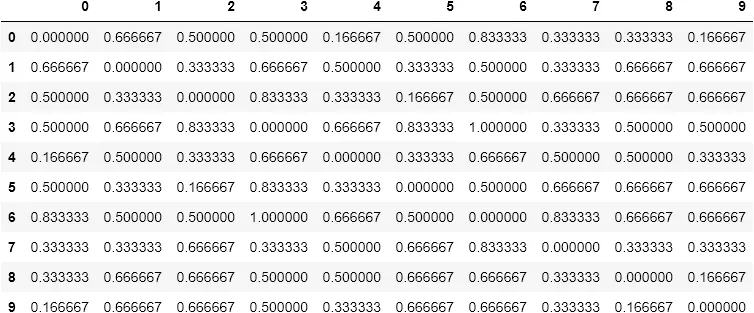
Part 3: Summary
Packages Used
- Pandas version=1.1.5
- Numpy version=1.19.5
- category_encoders=2.2.2
- math
In this blogpost we have defined a few similarity measures and implemented them in python. In the future we must learn to interpret them and understand when and where to use them.
Note the code for Lin similarity measure seem to not work well.
QUESTION2
ANS:
Problem Statement :
To build a simple K-Means model for clustering the car data into different groups.
Data details
==========================================
1. Title: Car Evaluation Database==========================================
The dataset is available at “http://archive.ics.uci.edu/ml/datasets/Car+Evaluation”
2. Sources:
(a) Creator: Marko Bohanec
(b) Donors: Marko Bohanec ([email protected])
Blaz Zupan ([email protected])
(c) Date: June, 19973. Past Usage:
The hierarchical decision model, from which this dataset is derived, was first presented in M. Bohanec and V. Rajkovic: Knowledge acquisition and explanation for multi-attribute decision making. In 8th Intl Workshop on Expert Systems and their Applications, Avignon, France. pages 59-78, 1988.
Within machine-learning, this dataset was used for the evaluation of HINT (Hierarchy INduction Tool), which was proved to be able to completely reconstruct the original hierarchical model. This, together with a comparison with C4.5, is presented in B. Zupan, M. Bohanec, I. Bratko, J. Demsar: Machine learning by function decomposition. ICML-97, Nashville, TN. 1997 (to appear)
4. Relevant Information Paragraph:
Car Evaluation Database was derived from a simple hierarchical decision model originally developed for the demonstration of DEX(M. Bohanec, V. Rajkovic: Expert system for decision making. Sistemica 1(1), pp. 145-157, 1990.). The model evaluates cars according to the following concept structure:
CAR car acceptability
. PRICE overall price
. . buying buying price
. . maint price of the maintenance
. TECH technical characteristics
. . COMFORT comfort
. . . doors number of doors
. . . persons capacity in terms of persons to carry
. . . lug_boot the size of luggage boot
. . safety estimated safety of the car
Input attributes are printed in lowercase. Besides the target concept (CAR), the model includes three intermediate concepts: PRICE, TECH, COMFORT. Every concept is in the original model related to its lower level descendants by a set of examples (for these examples sets see http://www-ai.ijs.si/BlazZupan/car.html).
The Car Evaluation Database contains examples with the structural information removed, i.e., directly relates CAR to the six input attributes: buying, maint, doors, persons, lug_boot, safety.
Because of known underlying concept structure, this database may be particularly useful for testing constructive induction and structure discovery methods.
5. Number of Instances: 1728
(instances completely cover the attribute space)
6. Number of Attributes: 6
7. Attribute Values:
buying v-high, high, med, low
maint v-high, high, med, low
doors 2, 3, 4, 5-more
persons 2, 4, more
lug_boot small, med, big
safety low, med, high
8. Missing Attribute Values: none
9. Class Distribution (number of instances per class)
class N N[%]
—————————–
unacc 1210 (70.023 %)
acc 384 (22.222 %)
good 69 ( 3.993 %)
v-good 65 ( 3.762 %)
Tools to be used :
Numpy,pandas,scikit-learn
Python Implementation with code :
Import necessary libraries
Import the necessary modules from specific libraries.
Load the data set
Use pandas module to read the bike data from the file system. Check few records of the dataset.
The train data set has 1728 rows and 7 columns.
There are no missing values in the dataset
The target variable is marked as class in the dataframe. The values are present in string format. However the algorithm requires the variables to be coded into its equivalent integer codes. We can convert the string categorical values into a integer code using factorize method of the pandas library.
Let’s check the encoded values now.
As we can see the values has been encoded into 4 different numeric labels.
Identify the predictor variables and encode any string variables to equivalent integer codes
Everything is now converted in integer form.
Select the predictor feature and select the target variable
In clustering there is no target variable as such. However clustering helps us to find a cluster which can be used as weak labels. These weak labels can bootstrap our supervised learning.
This technique is widely used for semi-supervised learning.
We need not worry about it as of now. You can just consider that y value will be used to validate the accuracy of weak labeling going ahead.
Check few parameters of the learnt cluster (Model parameters study):
Check the cluster centroids or means :
It should be 4 vectors or a matrix with 4 rows since the number of clusters we have fitted is 4.
Let’s check
he KMeans algorithm clusters data by trying to separate samples in n groups of equal variance, minimizing a criterion known as the inertia or within-cluster sum-of-squares Inertia, or the within-cluster sum of squares criterion, can be recognized as a measure of how internally coherent clusters are.
The k-means algorithm divides a set of N samples X into K disjoint clusters C, each described by the mean j of the samples in the cluster. The means are commonly called the cluster “centroids”.
The K-means algorithm aims to choose centroids that minimise the inertia, or within-cluster sum of squared criterion:
Inertia is not a normalized metric: we just know that lower values are better and zero is optimal. But in very high-dimensional spaces, Euclidean distances tend to become inflated (this is an instance of the so-called “curse of dimensionality”). Running a dimensionality reduction algorithm such as PCA prior to k-means clustering can alleviate this problem and speed up the computations.
We have achieved a weak classification accuracy of 26% by our unsupervised model. Not Bad.
!!!
How do we know value of optimal value of K
The value of k basically means that in how many clusters you can separate out the most homogeneous data. Choosing a large value of K will lead to greater amount of execution time. Selecting the small value of K might or might not give a good fit. There is no such guaranteed way to find the best value of K. However we can run few experiments and find the value of each model’s inertia and plot it on a graph. This plot is also known as elbow plot. We basically try to find the value of k from where there is major shift in value of inertia.
Let’s plot the graph
By the plot we can see that there is a kink at k=2. Hence k =2 can be considered as good number of cluster to cluster this data.
Let’s check the inertia and weak classification with number of cluster = 2.
Woah !!! our weak labeling is as good as a weak supervised classification model.
Pros and Cons
Time Complexity
K-means is linear in the number of data objects i.e. O(n), where n is the number of data objects. The time complexity of most of the hierarchical clustering algorithms is quadratic i.e. O(n2). Therefore, for the same amount of data, hierarchical clustering will take quadratic amount of time. Imagine clustering 1 million records?
Shape of Clusters
K-means works well when the shape of clusters are hyper-spherical (or circular in 2 dimensions). If the natural clusters occurring in the dataset are non-spherical then probably K-means is not a good choice.
Repeatability
K-means starts with a random choice of cluster centers, therefore it may yield different clustering results on different runs of the algorithm. Thus, the results may not be repeatable and lack consistency. However, with hierarchical clustering, you will most definitely get the same clustering results.
Off course, K-means clustering requires prior knowledge of K (or number of clusters), whereas in hierarchical clustering you can stop at whatever level (or clusters) you wish.