Supervised Learning - Classification Week 7 Challenge
QUESTIONS1
ANS:
Support Vector Machine
Pros & Cons
1- Thrives in High Dimension
When data has high dimension (think 1000+ to infinity features) a Support Vector Machine with the right settings (right kernel choice etc.) can be the way to go and produce really accurate results.
2- Kernel Flexibility
If you're a hands-on person who likes to learn and understand the intricacies of systems then you might actually enjoy the highly integrated kernel-world of Support Vector Machines.
Support Vector Machines are all about choosing the right kernel with the right parameters and this can provide lots of flexibility
and a potent toolset.
Linear kernels, non-linear kernels, polynomial kernels, RBF, sigmoid and gaussian kernels all have an edge in solving supervised machine learning problems with SVMs or SVRs.
3- Fast Prediction
Support Vector Machines may be relatively sluggish when it comes to training especially with large datasets, however, when it comes to prediction they are quite fast.
SVMs handle dataset as a whole at once and in this sense it's not an incremental approach. This means whole data is taken to RAM of a computer during training. Once it's done prediction becomes a breeze.
4- Both Classification and Regression Skills
SVMs can be used to both classify data and also predict continuous numerical values. Regression variance of Support Vector Machines are usually called SVR (Support Vector Regression)
support vector machine
Disadvantages
1- Advanced Settings
Although random forests have numerous optimization parameters too it's not so easy to make huge mistakes with them, but when it comes to Support Vector Machines, correct parameters can define the line between misery and victory.
This makes Support Vector Machines difficult to implement sometimes.
2- Suitable for Small Dataset
Support Vector Machines don't have a scalable nature and they don't work that well with mid-size or large datasets.
3)Costly Computation
SVMs are not the most efficient algorithms and it can be quite costly computationally to train them. (When applied with kernels and especially with non-linear kernels)
4- Feature Vectors Required
You can't just work on any problems with SVM Machine Learning Algorithms.
Dataset in hand will already need have feature vectors or you will need to pre-process to extract feature vectors which might not always be easy or possible.
5- Low Interpretability
Support Vector Machines don't provide very sophisticated and interpretable reports that can be interpreted in an easy fashion.
Lack of probability estimates also is another drawback of this machine learning algorithm.
6- Overfitting Risk
Overfitting is another potential side effect of Support Vector Machines and it can be quite difficult to detect or fix at times.
7- Scaling Neccessity
This is not necessarily a con but something that comes with Support Vector Machines and creates additional tasks and maybe you'd rather not deal with extra data preparation techniques.
Scaling is an important fundamental step when working with SVMs otherwise features with higher nominal values will dominate the decision-making process while calculating the distance between the plane and support vectors.
wrap-up
Support Vector Machine Pros & Cons Summary
Why Support Vector Machines?
However, in so many aspects Support Vector Machines face serious competition.
Concerning supervised machine learning space, SVMs can deal with linear as well as non-linear problems, they can also do classification as well as regression. Although accuracy wise they perform quite well, they don't produce very interpretable results.
Although they are good at handling large numbers of features they struggle with computation resources when data gets big.
It's probably safe to conclude that Support Vector Machines happily live in a specific but limited zone where data is considerably small (think up to 20.000 rows) and features are plenty. And, don't forget to really optimize the hyper-parameters and their parameters!
Easy Interpretation
This gotta be the biggest edge of Decision Trees. They just give easy, readable outputs.
Easy Data Prep
Data prep is easy with Decision Trees on so many levels. (missing data is ok,no normalization, no scaling etc.)
Computation Cost
Compared to some algorithms such as random forests, decision trees are a lighter alternative.
Parameter Complexity
Decision Trees come with a learning curve especially if you want to get hands-on with them. There are lots of important parameters that can make a big difference.
Relatively Slow
Despite its edge on Random Forests, Decision Trees are computationally expensive in general.
Limited Power
Decision tree can be limited in its accuracy and tackling complex data.
QUESTION2
ANS:
Implementing SVM for Classification and finding Accuracy in Python
using datasets- Wine, Boston and Diabetes
Problem Statement: Implement SVM for performing classification and find its accuracy on the given data. (Using Python) (Datasets — Wine, Boston and Diabetes)
Link to the program and Datasets is given below
SVM stands for Support Vector Machine. SVM is a supervised machine learning algorithm that is commonly used for classification and regression challenges. Common applications of the SVM algorithm are Intrusion Detection System, Handwriting Recognition, Protein Structure Prediction, Detecting Steganography in digital images, etc.
In the SVM algorithm, each point is represented as a data item within the n-dimensional space where the value of each feature is the value of a specific coordinate.
After plotting, classification has been performed by finding hype-plane which differentiates two classes. Refer below image to understand this concept.
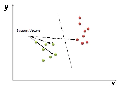
Support Vector Machine algorithm is mainly used to solve classification problems. Support vectors are nothing but the coordinates of each data item. Support Vector Machine is a frontier that differentiates two classes using hyper-plane.
Working of Support Vector Algorithm
SVM works by mapping data to a high-dimensional feature space so that data points can be categorized, even when the data are not otherwise linearly separable. A separator between the categories is found, then the data are transformed in such a way that the separator could be drawn as a hyperplane.
Support Vector machines have some special data points which we call “Support Vectors” and a separating hyperplane which is known as “Support Vector Machine”. So, essentially SVM is a frontier that best segregates the classes. Support Vectors are the data points nearest to the hyperplane, the points of our data set which if removed, would alter the position of the dividing hyperplane. As we can see that there can be many hyperplanes which can segregate the two classes, the hyperplane that we would choose is the one with the highest margin.
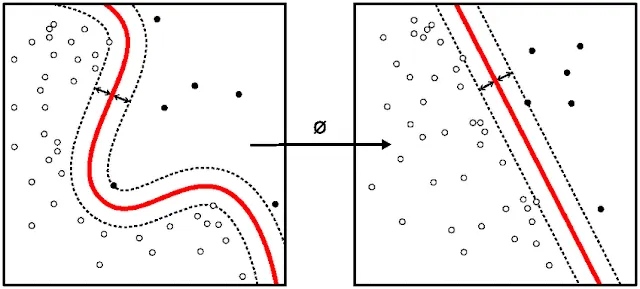
The mathematical function used for the transformation is known as the kernel function. SVM supports the following kernel types:
• Linear
• Polynomial
• Radial basis function (RBF)
• Sigmoid
Program on SVM for performing classification and finding its accuracy on the given data:
Step 1: Import libraries
First, we will import the libraries needed for our program.
- We import svm and datasets from the sklearn Library
- Numpy for carrying out efficient mathematical computations
- accuracy_score from sklearn.metrics to predict the accuracy of the model and from sklearn.model_selection import train_test_split for splitting the data into a training set and testing set
Step 2: Add datasets, insert the desired number of features and train the model
Here is the code for importing inbuilt dataset. “iris” is the variable name in which we will be loading our required dataset.
We can also import the dataset from the location it is stored on your computer to a new variable.The pd.read_csv is used to read the csv file (dataset file). The following code shows the syntax:-
Iris = pd.read_csv(‘C:/Users/Kshitij Ved/Desktop/Iris.csv’)
In the next step X variable is loaded with iris.data[:, :2], in this we only take the first two features as input for training.
And the Y variable is loaded with iris.target, that is the output of the original data.
Then we Split arrays or matrices into a random train and test subset using train_test_split(). We provide the proportion of data to use as a test set and we can provide the parameter random_state, which is used to ensure repeatable results. Test_size is used to decide how much data to be given for testing to the model.
Moving along, we are now going to define our classifier…
We will be using the SVC (support vector classifier) SVM (support vector machine). Our kernel is going to be linear, and C is equal to 1. C is a valuation of “how badly” you want to properly classify, or fit, everything. We are going to just stick with 1 for now, which is a nice default parameter.
Step 3: Predicting the output and printing the accuracy of the model
In the next step we use the clf.predict(x_test), that is the classifier to predict the test results and then we print the accuracy score, In the above example, 76.31578947368422 is the predicted value of the model when we load iris as the data set.
Step 4: Finally plotting the classifier for our program
In this step, we will be plotting our classifier. Here the np.meshgrid() function is used to create a rectangular grid out of two given one-dimensional arrays representing the Cartesian indexing or Matrix indexing.
NumPy provides the reshape() function on the NumPy array object that can be used to reshape the data. In the case of reshaping a one-dimensional array into a two-dimensional array with one column, the tuple would be the shape of the array as the first dimension and 1 for the second dimension.
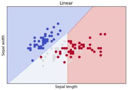
plt.scatter() is used to plot the points on the graph and plt.show() displays the graph.