Supervised Learning - Classification Week 9 Challenge
QUESTION1
ANS:
What is Neural Networks?
The computing systems inspired by biological neural networks to perform different tasks with a huge amount of data involved is called artificial neural networks or ANN. Different algorithms are used to understand the relationships in a given set of data to produce the best results from the changing inputs. The network is trained to produce the desired outputs, and different models are used to predict the future results with the data. The nodes are interconnected so that it works like a human brain. Different correlations and hidden patterns in raw data are used to cluster and classify the data.
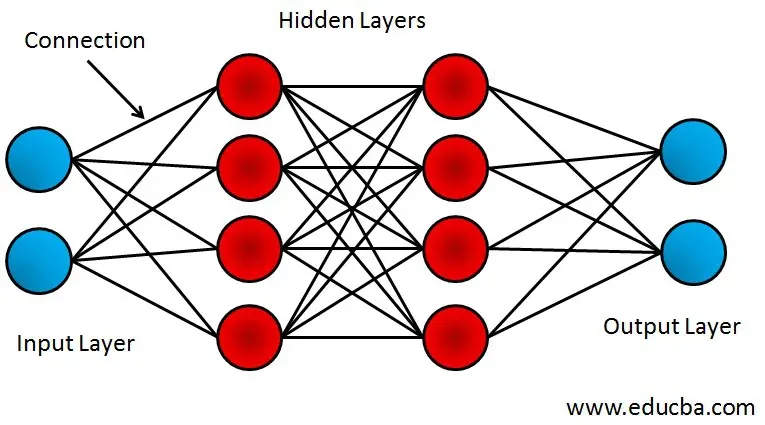
Understanding Neural Network
Neural networks are trained and taught just like a child’s developing brain is trained. They cannot be programmed directly for a particular task. Instead, they are trained in such a manner so that they can adapt according to the changing input.
There are three methods or learning paradigms to teach a neural network.
- Supervised Learning
- Reinforcement Learning
- Unsupervised Learning
1. Supervised Learning
As the name suggests, supervised learning means in the presence of a supervisor or a teacher. It means a set of a labeled data sets is already present with the desired output, i.e. the optimum action to be performed by the neural network, which is already present for some data sets. The machine is then given new data sets to analyze the training data sets and to produce the correct output.
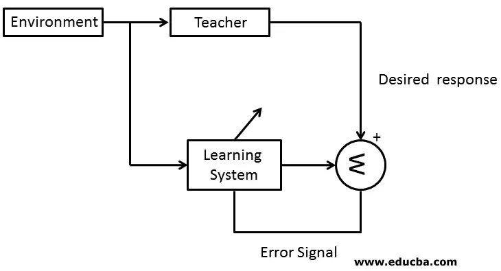
It is a closed feedback system, but the environment is not in the loop.
2. Reinforcement Learning
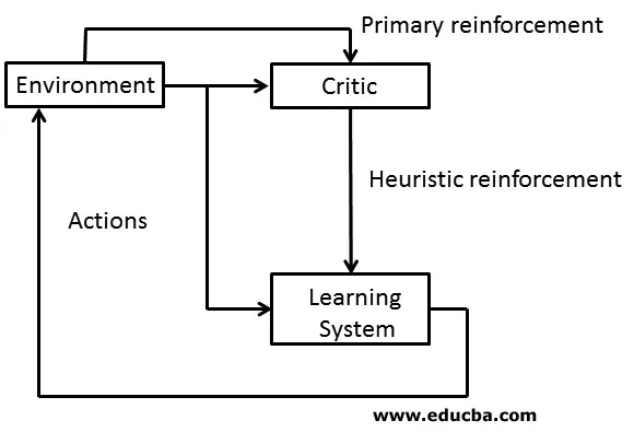
In this, learning of input-output mapping is done by continuous interaction with the environment to minimise the scalar index of performance. In this, instead of a teacher, a critic converts the primary reinforcement signal, i.e. the scalar input received from the environment, into a heuristic reinforcement signal (higher quality reinforcement signal) scalar input.
This learning aims to minimize the cost to go function, i.e. the expected cumulative cost of actions taken over a sequence of steps.
3. Unsupervised Learning
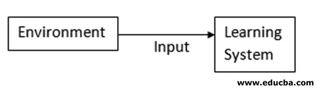
As the name suggests, there is no teacher or supervisor available. In this, the data is neither labeled nor classified, and no prior guidance is available to the neural network. In this, the machine has to group the provided data sets according to the similarities, differences, and patterns without any training provided beforehand.
Working with Neural Network
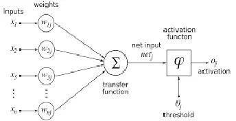
The neural network is a weighted graph where nodes are the neurons, and edges with weights represent the connections. It takes input from the outside world and is denoted by x(n).
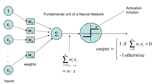
Each input is multiplied by its respective weights, and then they are added. A bias is added if the weighted sum equates to zero, where bias has input as 1 with weight b. Then this weighted sum is passed to the activation function. The activation function limits the amplitude of the output of the neuron. There are various activation functions like the Threshold function, Piecewise linear function, or Sigmoid function.
Architecture of Neural Network
There are basically three types of architecture of the neural network.
- Single Layer feedforward network
- Multi-Layer feedforward network
- Recurrent network
1. Single- Layer Feedforward Network
In this, we have an input layer of source nodes projected on an output layer of neurons. This network is a feedforward or acyclic network. It is termed a single layer because it only refers to the computation neurons of the output layer. No computation is performed on the input layer; hence it is not counted.
2. Multi-Layer Feedforward Network
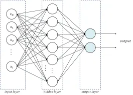
In this, there are one or more hidden layers except for the input and output layers. The nodes of this layer are called hidden neurons or hidden units. The role of the hidden layer is to intervene between the output and the external input. The input layer nodes supply the input signal to the second layer’s nodes, i.e. the hidden layer, and the output of the hidden layer acts as an input for the next layer, which continues for the rest of the network.
3. Recurrent Networks
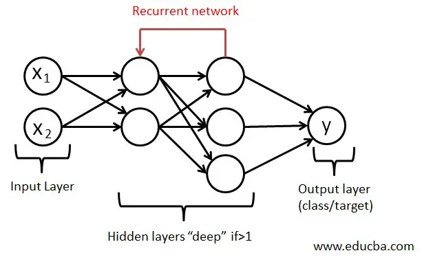
A recurrent is almost similar to a feedforward network. The major difference is that it at least has one feedback loop. There might be zero or more hidden layers, but at least one feedback loop will be there.
Advantages of Neural Network
Given below are the advantages mentioned:
- Can work with incomplete information once trained.
- Have the ability of fault tolerance.
- Have a distributed memory
- Can make machine learning.
- Parallel processing.
- Stores information on an entire network.
- Can learn non-linear and complex relationships.
- Ability to generaize, i.e. can infer unseen relationships after learning from some prior relationships.
Required Neural Network Skills
Given below are the required neural network skills:
- Knowledge of applied maths and algorithms.
- Probability and statistics.
- Distributed computing.
- Fundamental programming skills.
- Data modeling and evaluation.
- Software engineering and system design.
Why should we use Neural Networks?
- It helps to model the nonlinear and complex relationships of the real world.
- They are used in pattern recognition because they can generalize.
- They have many applications like text summarization, signature identification, handwriting recognition, and many more.
- It can model data with high volatility.
Neural Networks Scope
It has a wide scope in the future. Researchers are constantly working on new technologies based on neural networks. Everything is converting into automation; hence they are very much efficient in dealing with changes and can adapt accordingly. Due to an increase in new technologies, there are many job openings for engineers and neural network experts. Hence in the future also neural networks will prove to be a major job provider.
How this Technology will help you in Career Growth
There is huge career growth in the field of neural networks. The average salary of a neural network engineer ranges from $33,856 to $153,240 per year approximately.
Conclusion – What is Neural Networks?
There is a lot to gain from neural networks. They can learn and adapt according to the changing environment. Moreover, they contribute to other areas as well as in the field of neurology and psychology. Hence there is a huge scope of neural networks in today’s time as well as in the future.
QUESTION2
ANS:
Deep Learning
What is deep learning?
Deep learning is a subset of machine learning, which is essentially a neural network with three or more layers. These neural networks attempt to simulate the behavior of the human brain—albeit far from matching its ability—allowing it to “learn” from large amounts of data. While a neural network with a single layer can still make approximate predictions, additional hidden layers can help to optimize and refine for accuracy.
Deep learning drives many artificial intelligence (AI) applications and services that improve automation, performing analytical and physical tasks without human intervention. Deep learning technology lies behind everyday products and services (such as digital assistants, voice-enabled TV remotes, and credit card fraud detection) as well as emerging technologies (such as self-driving cars).
Deep learning vs. machine learning
If deep learning is a subset of machine learning, how do they differ? Deep learning distinguishes itself from classical machine learning by the type of data that it works with and the methods in which it learns.
Machine learning algorithms leverage structured, labeled data to make predictions—meaning that specific features are defined from the input data for the model and organized into tables. This doesn’t necessarily mean that it doesn’t use unstructured data; it just means that if it does, it generally goes through some pre-processing to organize it into a structured format.
Deep learning eliminates some of data pre-processing that is typically involved with machine learning. These algorithms can ingest and process unstructured data, like text and images, and it automates feature extraction, removing some of the dependency on human experts. For example, let’s say that we had a set of photos of different pets, and we wanted to categorize by “cat”, “dog”, “hamster”, et cetera. Deep learning algorithms can determine which features (e.g. ears) are most important to distinguish each animal from another. In machine learning, this hierarchy of features is established manually by a human expert.
Then, through the processes of gradient descent and backpropagation, the deep learning algorithm adjusts and fits itself for accuracy, allowing it to make predictions about a new photo of an animal with increased precision.
Machine learning and deep learning models are capable of different types of learning as well, which are usually categorized as supervised learning, unsupervised learning, and reinforcement learning. Supervised learning utilizes labeled datasets to categorize or make predictions; this requires some kind of human intervention to label input data correctly. In contrast, unsupervised learning doesn’t require labeled datasets, and instead, it detects patterns in the data, clustering them by any distinguishing characteristics. Reinforcement learning is a process in which a model learns to become more accurate for performing an action in an environment based on feedback in order to maximize the reward.
For a deeper dive on the nuanced differences between the different technologies, see "AI vs. Machine Learning vs. Deep Learning vs. Neural Networks: What’s the Difference?"
For a closer look at the specific differences between supervised and unsupervised learning, see "Supervised vs. Unsupervised Learning: What's the Difference?"
How deep learning works
Deep learning neural networks, or artificial neural networks, attempts to mimic the human brain through a combination of data inputs, weights, and bias. These elements work together to accurately recognize, classify, and describe objects within the data.
Deep neural networks consist of multiple layers of interconnected nodes, each building upon the previous layer to refine and optimize the prediction or categorization. This progression of computations through the network is called forward propagation. The input and output layers of a deep neural network are called visible layers. The input layer is where the deep learning model ingests the data for processing, and the output layer is where the final prediction or classification is made.
Another process called backpropagation uses algorithms, like gradient descent, to calculate errors in predictions and then adjusts the weights and biases of the function by moving backwards through the layers in an effort to train the model. Together, forward propagation and backpropagation allow a neural network to make predictions and correct for any errors accordingly. Over time, the algorithm becomes gradually more accurate.
The above describes the simplest type of deep neural network in the simplest terms. However, deep learning algorithms are incredibly complex, and there are different types of neural networks to address specific problems or datasets. For example,
- Convolutional neural networks (CNNs), used primarily in computer vision and image classification applications, can detect features and patterns within an image, enabling tasks, like object detection or recognition. In 2015, a CNN bested a human in an object recognition challenge for the first time.
- Recurrent neural network (RNNs) are typically used in natural language and speech recognition applications as it leverages sequential or times series data.
Deep learning applications
Real-world deep learning applications are a part of our daily lives, but in most cases, they are so well-integrated into products and services that users are unaware of the complex data processing that is taking place in the background. Some of these examples include the following:
Law enforcement
Deep learning algorithms can analyze and learn from transactional data to identify dangerous patterns that indicate possible fraudulent or criminal activity. Speech recognition, computer vision, and other deep learning applications can improve the efficiency and effectiveness of investigative analysis by extracting patterns and evidence from sound and video recordings, images, and documents, which helps law enforcement analyze large amounts of data more quickly and accurately.
Financial services
Financial institutions regularly use predictive analytics to drive algorithmic trading of stocks, assess business risks for loan approvals, detect fraud, and help manage credit and investment portfolios for clients.
Customer service
Many organizations incorporate deep learning technology into their customer service processes. Chatbots—used in a variety of applications, services, and customer service portals—are a straightforward form of AI. Traditional chatbots use natural language and even visual recognition, commonly found in call center-like menus. However, more sophisticated chatbot solutions attempt to determine, through learning, if there are multiple responses to ambiguous questions. Based on the responses it receives, the chatbot then tries to answer these questions directly or route the conversation to a human user.
Virtual assistants like Apple's Siri, Amazon Alexa, or Google Assistant extends the idea of a chatbot by enabling speech recognition functionality. This creates a new method to engage users in a personalized way.
Healthcare
The healthcare industry has benefited greatly from deep learning capabilities ever since the digitization of hospital records and images. Image recognition applications can support medical imaging specialists and radiologists, helping them analyze and assess more images in less time.
Deep learning hardware requirements
Deep learning requires a tremendous amount of computing power. High performance graphical processing units (GPUs) are ideal because they can handle a large volume of calculations in multiple cores with copious memory available. However, managing multiple GPUs on-premises can create a large demand on internal resources and be incredibly costly to scale.
QUESTION3
ANS:
Activation functions in Neural Networks
- Difficulty Level : Basic
- Last Updated : 08 Oct, 2020
It is recommended to understand what is a neural network before reading this article. In The process of building a neural network, one of the choices you get to make is what activation function to use in the hidden layer as well as at the output layer of the network. This article discusses some of the choices.
Elements of a Neural Network :-
Input Layer :- This layer accepts input features. It provides information from the outside world to the network, no computation is performed at this layer, nodes here just pass on the information(features) to the hidden layer.
Hidden Layer :- Nodes of this layer are not exposed to the outer world, they are the part of the abstraction provided by any neural network. Hidden layer performs all sort of computation on the features entered through the input layer and transfer the result to the output layer.
Output Layer :- This layer bring up the information learned by the network to the outer world.
What is an activation function and why to use them?
Definition of activation function:- Activation function decides, whether a neuron should be activated or not by calculating weighted sum and further adding bias with it. The purpose of the activation function is to introduce non-linearity into the output of a neuron.
Explanation :-
We know, neural network has neurons that work in correspondence of weight, bias and their respective activation function. In a neural network, we would update the weights and biases of the neurons on the basis of the error at the output. This process is known as back-propagation. Activation functions make the back-propagation possible since the gradients are supplied along with the error to update the weights and biases.
Why do we need Non-linear activation functions :-
A neural network without an activation function is essentially just a linear regression model. The activation function does the non-linear transformation to the input making it capable to learn and perform more complex tasks.
Mathematical proof :-
Suppose we have a Neural net like this :-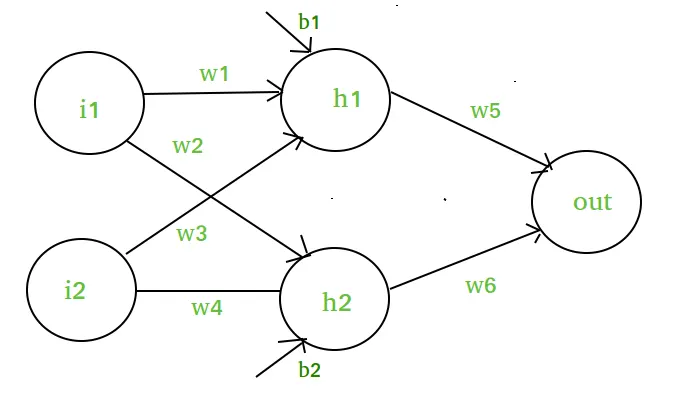
Elements of the diagram :-
Hidden layer i.e. layer 1 :-
z(1) = W(1)X + b(1)
a(1) = z(1)
Here,
- z(1) is the vectorized output of layer 1
- W(1) be the vectorized weights assigned to neurons
of hidden layer i.e. w1, w2, w3 and w4- X be the vectorized input features i.e. i1 and i2
- b is the vectorized bias assigned to neurons in hidden
layer i.e. b1 and b2- a(1) is the vectorized form of any linear function.
(Note: We are not considering activation function here)
Layer 2 i.e. output layer :-
//  Note : Input for layer
//   2 is output from layer 1
z(2) = W(2)a(1) + b(2)
a(2) = z(2)
Calculation at Output layer:
// Putting value of z(1) here

z(2) = (W(2) * [W(1)X + b(1)]) + b(2)

z(2) = [W(2) * W(1)] * X + [W(2)*b(1) + b(2)]

Let,
    [W(2) * W(1)] = W
    [W(2)*b(1) + b(2)] = b

Final output : z(2) = W*X + b
Which is again a linear function
This observation results again in a linear function even after applying a hidden layer, hence we can conclude that, doesn’t matter how many hidden layer we attach in neural net, all layers will behave same way because the composition of two linear function is a linear function itself. Neuron can not learn with just a linear function attached to it. A non-linear activation function will let it learn as per the difference w.r.t error.
Hence we need activation function.
VARIANTS OF ACTIVATION FUNCTION :-
1). Linear Function :-
- Equation : Linear function has the equation similar to as of a straight line i.e. y = ax
- No matter how many layers we have, if all are linear in nature, the final activation function of last layer is nothing but just a linear function of the input of first layer.
- Range : -inf to +inf
- Uses : Linear activation function is used at just one place i.e. output layer.
- Issues : If we will differentiate linear function to bring non-linearity, result will no more depend on input “x” and function will become constant, it won’t introduce any ground-breaking behavior to our algorithm.
For example : Calculation of price of a house is a regression problem. House price may have any big/small value, so we can apply linear activation at output layer. Even in this case neural net must have any non-linear function at hidden layers.
2). Sigmoid Function :-
- It is a function which is plotted as ‘S’ shaped graph.
- Equation :
A = 1/(1 + e-x) - Nature : Non-linear. Notice that X values lies between -2 to 2, Y values are very steep. This means, small changes in x would also bring about large changes in the value of Y.
- Value Range : 0 to 1
- Uses : Usually used in output layer of a binary classification, where result is either 0 or 1, as value for sigmoid function lies between 0 and 1 only so, result can be predicted easily to be 1 if value is greater than 0.5 and 0 otherwise.
3). Tanh Function :- The activation that works almost always better than sigmoid function is Tanh function also knows as Tangent Hyperbolic function. It’s actually mathematically shifted version of the sigmoid function. Both are similar and can be derived from each other.
- Equation :-
f(x) = tanh(x) = 2/(1 + e-2x) - 1
OR
tanh(x) = 2 * sigmoid(2x) - 1
- Value Range :- -1 to +1
- Nature :- non-linear
- Uses :- Usually used in hidden layers of a neural network as it’s values lies between -1 to 1 hence the mean for the hidden layer comes out be 0 or very close to it, hence helps in centering the data by bringing mean close to 0. This makes learning for the next layer much easier.
4). RELU :- Stands for Rectified linear unit. It is the most widely used activation function. Chiefly implemented in hidden layers of Neural network.
- Equation :- A(x) = max(0,x). It gives an output x if x is positive and 0 otherwise.
- Value Range :- [0, inf)
- Nature :- non-linear, which means we can easily backpropagate the errors and have multiple layers of neurons being activated by the ReLU function.
- Uses :- ReLu is less computationally expensive than tanh and sigmoid because it involves simpler mathematical operations. At a time only a few neurons are activated making the network sparse making it efficient and easy for computation.
In simple words, RELU learns much faster than sigmoid and Tanh function.
5). Softmax Function :- The softmax function is also a type of sigmoid function but is handy when we are trying to handle classification problems.
- Nature :- non-linear
- Uses :- Usually used when trying to handle multiple classes. The softmax function would squeeze the outputs for each class between 0 and 1 and would also divide by the sum of the outputs.
- Output:- The softmax function is ideally used in the output layer of the classifier where we are actually trying to attain the probabilities to define the class of each input.
CHOOSING THE RIGHT ACTIVATION FUNCTION
- The basic rule of thumb is if you really don’t know what activation function to use, then simply use RELU as it is a general activation function and is used in most cases these days.
- If your output is for binary classification then, sigmoid function is very natural choice for output layer.
Foot Note :-
QUESTION4
The activation function does the non-linear transformation to the input making it capable to learn and perform more complex tasks. - ANS:
7 Types of Activation Functions in Neural Network
Introduction
The neural network activation functions, in general, are the most significant component of deep learning, they are fundamentally used for determining the output of deep learning models, its accuracy, and performance efficiency of the training model that can design or divide a huge scale neural network.
Activation functions have left considerable effects on the ability of neural networks to converge and convergence speed, don’t you want to how? Let’s continue with an introduction to the activation function, types of activation functions & their importance and limitations through this blog.
What is the activation function?
Activation function defines the output of input or set of inputs or in other terms defines node of the output of node that is given in inputs.
They basically decide to activate or deactivate neurons to get the desired output. It also performs a nonlinear transformation on the input to get better results on a complex neural network.
Activation function also helps to normalize the output of any input in the range between 1 to -1. Activation function must be efficient and it should reduce the computation time because the neural network sometimes trained on millions of data points.
Activation function basically decides in any neural network that given input or receiving information is relevant or it is irrelevant. Let's take an example to understand better what is a neuron and how activation function bounds the output value to some limit.
The neuron is basically is a weighted average of input, then this sum is passed through an activation function to get an output.
Y = ∑ (weights*input + bias)
Here Y can be anything for a neuron between range -infinity to +infinity. So, we have to bound our output to get the desired prediction or generalized results.
Y = Activation function(∑ (weights*input + bias))
So, we pass that neuron to activation function to bound output values.
Why do we need Activation Functions?
Without activation function, weight and bias would only have a linear transformation, or neural network is just a linear regression model, a linear equation is polynomial of one degree only which is simple to solve but limited in terms of ability to solve complex problems or higher degree polynomials.
But opposite to that, the addition of activation function to neural network executes the non-linear transformation to input and make it capable to solve complex problems such as language translations and image classifications.
In addition to that, Activation functions are differentiable due to which they can easily implement back propagations, optimized strategy while performing backpropagations to measure gradient loss functions in the neural networks.
Types of Activation Functions
We have divided all the essential neural networks in three major parts:
A. Binary step function
B. Linear function
C. Non linear activation function
A. Binary Step Neural Network Activation Function
1. Binary Step Function
This activation function very basic and it comes to mind every time if we try to bound output. It is basically a threshold base classifier, in this, we decide some threshold value to decide output that neuron should be activated or deactivated.
f(x) = 1 if x > 0 else 0 if x < 0
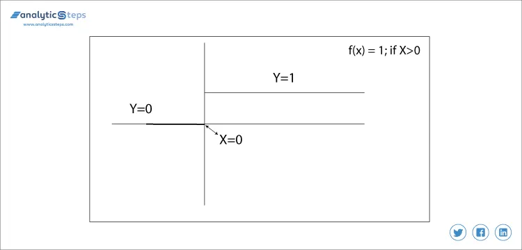
Binary step function
In this, we decide the threshold value to 0. It is very simple and useful to classify binary problems or classifier.
B. Linear Neural Network Activation Function
2. Linear Function
It is a simple straight line activation function where our function is directly proportional to the weighted sum of neurons or input. Linear activation functions are better in giving a wide range of activations and a line of a positive slope may increase the firing rate as the input rate increases.
In binary, either a neuron is firing or not. If you know gradient descent in deep learning then you would notice that in this function derivative is constant.
Y = mZ
Where derivative with respect to Z is constant m. The meaning gradient is also constant and it has nothing to do with Z. In this, if the changes made in backpropagation will be constant and not dependent on Z so this will not be good for learning.
In this, our second layer is the output of a linear function of previous layers input. Wait a minute, what have we learned in this that if we compare our all the layers and remove all the layers except the first and last then also we can only get an output which is a linear function of the first layer.
C. Non Linear Neural Network Activation Function
3. ReLU( Rectified Linear unit) Activation function
Rectified linear unit or ReLU is most widely used activation function right now which ranges from 0 to infinity, All the negative values are converted into zero, and this conversion rate is so fast that neither it can map nor fit into data properly which creates a problem, but where there is a problem there is a solution.
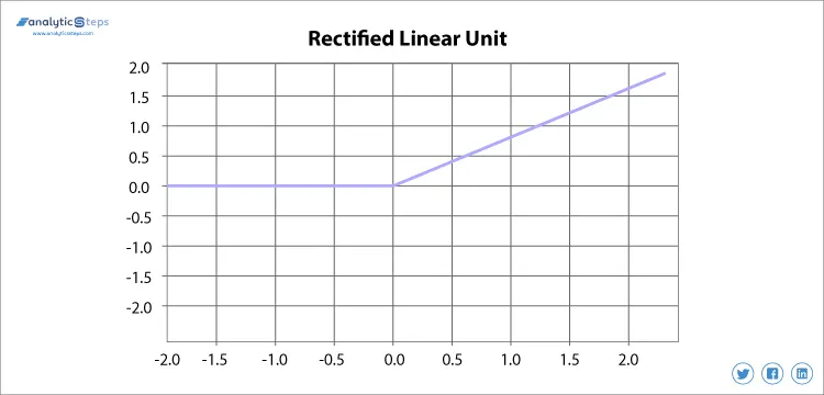
Rectified Linear Unit activation function
We use Leaky ReLU function instead of ReLU to avoid this unfitting, in Leaky ReLU range is expanded which enhances the performance.
4. Leaky ReLU Activation Function
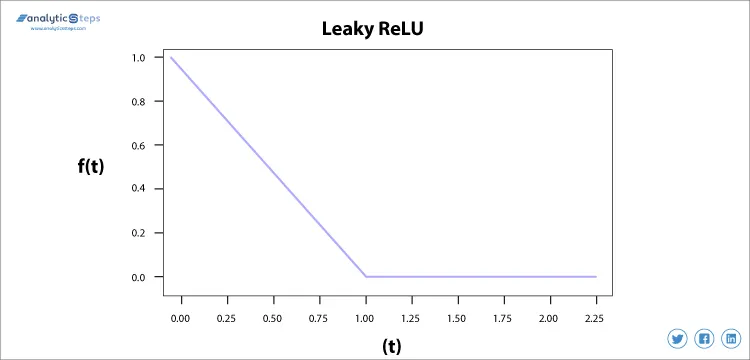
Leaky ReLU Activation Function
We needed the Leaky ReLU activation function to solve the ‘Dying ReLU’ problem, as discussed in ReLU, we observe that all the negative input values turn into zero very quickly and in the case of Leaky ReLU we do not make all negative inputs to zero but to a value near to zero which solves the major issue of ReLU activation function.
5. Sigmoid Activation Function
The sigmoid activation function is used mostly as it does its task with great efficiency, it basically is a probabilistic approach towards decision making and ranges in between 0 to 1, so when we have to make a decision or to predict an output we use this activation function because of the range is the minimum, therefore, prediction would be more accurate.
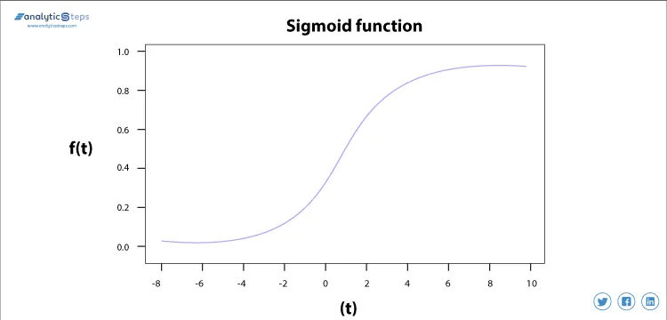
Sigmoid Activation function
The equation for the sigmoid function is
f(x) = 1/(1+e(-x) )
The sigmoid function causes a problem mainly termed as vanishing gradient problem which occurs because we convert large input in between the range of 0 to 1 and therefore their derivatives become much smaller which does not give satisfactory output. To solve this problem another activation function such as ReLU is used where we do not have a small derivative problem.
6. Hyperbolic Tangent Activation Function(Tanh)
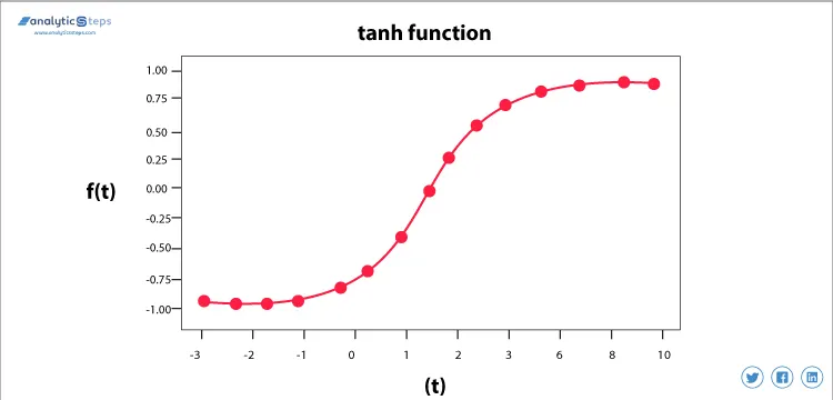
Tanh Activation function
This activation function is slightly better than the sigmoid function, like the sigmoid function it is also used to predict or to differentiate between two classes but it maps the negative input into negative quantity only and ranges in between -1 to 1.
7. Softmax Activation Function
Softmax is used mainly at the last layer i.e output layer for decision making the same as sigmoid activation works, the softmax basically gives value to the input variable according to their weight and the sum of these weights is eventually one.
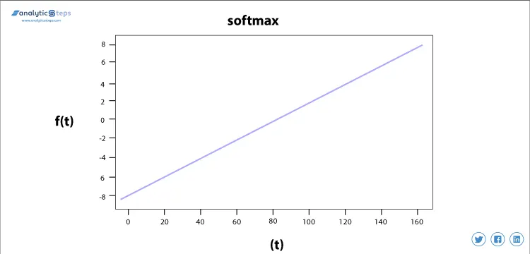
Softmax on Binary Classification
For Binary classification, both sigmoid, as well as softmax, are equally approachable but in case of multi-class classification problem we generally use softmax and cross-entropy along with it.
Conclusion
The activation functions are those significant functions that perform a non-linear transformation to the input and making it proficient to understand and executes more complex tasks. We have discussed majorly used activation functions with their limitation (if any), these activation functions are used for the same purpose but in different conditions.
QUESTION5
ANS:
What is backpropagation really doing?
Here we tackle backpropagation, the core algorithm behind how neural networks learn. If you followed the last two lessons or if you’re jumping in with the appropriate background, you know what a neural network is and how it feeds forward information.
Quick Recap
We’ve been looking at the classic example of recognizing handwritten digits. I’ve been showing a network with...
- An input layer of 784 neurons (which represent the pixel values of the image)
- Two hidden layers with 16 neurons each
- An output layer with 10 neurons (indicating the network’s choice of digit)
Our basic neural network has four layers: An input layer, an output layer, and two hidden layers in between.
We’ve also discussed gradient descent, so you should know that when people describe a network as “learning,” they mean finding the weights and biases that minimize a certain cost function.
We use gradient descent to walk downhill to a local minimum of the cost function.
To calculate the cost of a single training example, you take the output that the network gives, along with the output you wanted it to give, and you add up the squares of the differences between each component:
The cost for a single training example is the sum of the squares of the differences between the actual output and the desired output.
Doing this for all your tens of thousands of training examples, and averaging all the results, gives you the total cost of the network.
What is Backpropagation?
Remember, the negative gradient of the cost function is a 13,002-dimensional vector that tells us how to nudge all the weights and biases to decrease the cost most efficiently. Backpropagation, the topic of this lesson, is an algorithm for computing that negative gradient.
Thinking about the gradient vector as a direction in a 13,002-dimensional space is, to put it lightly, beyond the scope of our imaginations.
Direction in 13,002 dimensions?!?
So as we talked about in the previous lesson, it's helpful to consider it this way: The magnitude of each component of the gradient tells you how sensitive the cost function is to each corresponding weight and bias.
For example, let’s say you compute the negative gradient, using the process I’m about to describe, and the component associated with the weight on one edge comes out to be 3.2, while the component associated with some other edge is 0.1:
Suppose the entry of the gradient vector associated with one weight is 32x as large as the entry associated with some other weight.
The way to read this is that the cost function is 32 times more sensitive to changes to that first weight. So if you were to wiggle the value of that weight a bit, it’ll cause a change to the cost function 32 times greater than what the same wiggle to the second weight would cause.
Changing a weight that has a larger magnitude in the negative gradient vector has a bigger effect on the cost.
The Intuition for Backpropagation
When I first learned backpropagation, the most confusing aspect was just the notation and index chasing of it all.
There’s a lot of notation here. What does it all mean!?
For this article, let’s begin with a complete disregard for notation and instead step through the effect that each training example has on the weights and biases. Hopefully, these effects will feel intuitive so that by the time we return to the notation, it acts to articulate something you already know, rather than acting as a code to be decrypted.
Because the full cost function involves averaging a certain cost-per-example for all the tens of thousands of training examples, the way we adjust all the weights and biases for a single gradient descent step also depends on every single example. Or, rather, in principle it should, but for computational efficiency, we’ll do a little trick later to keep you from needing to hit every single example for every single step.
Right now, though, focus your attention on a single example, this image of a 2:
How can we adjust the weights and biases to improve the network’s performance on this image?
What effect does this one training example have on how the weights and biases should be adjusted?
Because the network is not yet well trained, the activations in that output layer are effectively random. That's no good; we want to change these activations so that they properly identify the digit 2.
But remember, we only have control over the weights and biases of the network. So we will have to nudge those weights and biases in a way that improves the output.
The activations in the output layer are trash, and we need to fix them by adjusting the weights and biases.
Although we can't directly change the activations, it’s helpful to keep track of what adjustments we wish to take place in this output layer.
Since we want the network to classify this as a 2, we want the digit 2 neuron’s value to be nudged up while all the others get nudged down:
Moreover, the sizes of these nudges should be proportional to how far off each output value is from the target. Neurons that are way off require big nudges, but neurons that are pretty close to correct only require little nudges.
Zooming in further, let’s focus on the one neuron whose activation we wish to increase:
Remember that its activation value (in this case 0.2) is defined as a weighted sum of all activations from the previous layer, plus a bias, which is then plugged into something like the sigmoid squishification or a ReLU:
So there are three avenues that can team up together to increase this activation:
- Increase the bias
- Increase the weights
- Change the activations from the previous layer
Changing the Bias
Changing the bias associated with a neuron is the simplest way to change its activation. Unlike changing the weights or the activations from the previous layer, the effect of a change to the bias on the weighted sum is constant and predictable.
Since we want to increase the activation of the digit-2 output neuron we've been discussing, how should its associated bias be adjusted? What about the biases associated with all the other output neurons for this training example?
Increase the bias associated with the digit-2 neuron and increase the biases associated with all the other neurons.
Increase the bias associated with the digit-2 neuron and decrease the biases associated with all the other neurons.
Decrease the bias associated with the digit-2 neuron and increase the biases associated with all the other neurons.
Decrease the bias associated with the digit-2 neuron and decrease the biases associated with all the other neurons.
Changing the Weights
How should the weights be adjusted? Notice, because they are being multiplied by the activations, the weights have differing levels of influence:
Changing the weights associated with large activation values will have a stronger effect than changing the weights associated with small activation values.
The connections with the brightest neurons from the preceding layer have the biggest effect since those weights are multiplied by larger activation values. So increasing one of those weights has a bigger influence on the cost function than increasing the weight of a connection with a dimmer neuron. (Again, this is all only insofar as this one training example is concerned.)
Remember, when we talk about gradient descent, we don’t just care about whether each component should be nudged up or down. We care about which ones give you the most bang for your buck.
To get the most bang for your buck, adjust the weights in proportion to their associated activations.
This, by the way, is at least somewhat reminiscent of a theory in neuroscience for how biological networks of neurons learn, Hebbian theory, often summed up in the phrase “neurons that fire together wire together.” Here, the biggest increases in weights—the biggest strengthening of connections—happens between neurons that are the most active and the ones which we wish to become more active.
In some sense, the neurons that fire while seeing a 2 get more strongly linked to those firing while thinking about a 2.
Connections are strengthened between neurons that should be activated at the same time.
The analogy is not perfect since the untrained network is not really “thinking” about a 2 when it sees this example; it’s more that the label on the training data is hardcoding what the network should be thinking about. Still, it’s satisfying to know that buried beneath all the calculus and linear algebra typically used to describe backpropagation, the actual changes happening to the weights with each training example mirror the ideas of Hebbian theory.
Changing the Activations
The third way we can help increase this neuron’s activation is by changing all the activations in the previous layer. Namely, if everything connected to that digit-2 neuron with a positive weight was brighter, and if everything connected with a negative weight was dimmer, that digit-2 neuron would be more active.
Similar to the weight changes, you’ll get the most bang for your buck by seeking changes proportional to the size of the corresponding weights:
Just like changing weights in proportion to activations, you get the most bang for your buck by increasing activations in proportion to their associated weights.
Of course, we cannot directly influence these activations. We only have control over the weights and biases. But just as with the last layer, it’s helpful to keep note of the desired changes.
We can’t influence the activations in the previous layer directly. But we can change the weights and biases that determine their values!
Remember, this is only what that one digit-2 output neuron wants. We also want all the other neurons in the last layer to become less active, and each of those other output neurons has its own influence on what should happen to the second-to-last layer.
We want to adjust all these other output neurons too, which means we will have many competing requests for changes to activations in the previous layer.
So the desire of this digit-2 neuron is added together with the desires of all the other nine neurons. Each has its own suggested nudge for that second-to-last layer, again in proportion to the corresponding weights and in proportion to how much each neuron needs to change.
It’s impossible to perfectly satisfy all these competing desires for activations in the second layer. The best we can do is add up all the desired nudges to find the overall desired change.
Here is where the idea of propagating backward comes in. By adding all these desired effects, you can get a list of the nudges you want to happen to this second-to-last layer. From there, you can recursively apply the same process to the relevant weights and biases determining those values, repeating this process as you move backward through the network.
Repeating for All Training Examples
Everything we just stepped through only records how a single training example wishes to nudge each of the many, many weights and biases.
So far we’ve only identified the nudges to the weights and biases that would improve our results for this digit 2. But we also need to account for all the other digits!
If we only listened to what that image of a 2 wanted, the network would ultimately be incentivized to just classify all images as a 2.
To zoom out a bit, you also go through this same backpropagation routine for every other training example, recording how each of them would like to change the weights and biases. Then you average together all those desired changes.
Each training example has its own desire for how the weights and biases should be adjusted, and with what relative strengths. By averaging together the desires of all training examples, we get the final result for how a given weight or bias should be changed in a single gradient descent step.
The collection of these averaged nudges to each weight and bias is, loosely speaking, the negative gradient of the cost function! Or at least something proportional to it.
The result of all this backpropagation is that we’ve found (something proportional to) the negative gradient!
I say “loosely speaking” only because I have yet to get quantitatively precise about these nudges. But if you understood each change I referenced above, why some are proportionally bigger than others, and how they all need to be added together, then you understand the mechanics for what backpropagation is actually doing.
Stochastic Gradient Descent
In practice, it takes computers an extremely long time to add up the influences of every single training example for every single gradient descent step. Instead, there’s a clever trick for speeding up the process in a way that involves more total gradient descent steps but much less time for each one.
Randomly shuffle your training data and divide it into a bunch of mini-batches, having, say, 100 training examples each.
Then you compute a gradient descent step according to each minibatch rather than the entire set of training examples. It won’t give you the actual gradient of the cost function, which depends on all the training data, so it’s not the most efficient step downhill. But each mini-batch gives a pretty good approximation, and if there are 100 minibatches, each step takes 1/100th of the total time. And after 100 steps, each piece of training data will have had its chance to influence the final result.
With these mini-batches, which only approximate the gradient, the process of gradient descent looks more like a drunk man stumbling aimlessly down a hill but taking quick steps rather than a carefully calculating man who takes slow, deliberate steps downhill.
Using mini-batches means our steps downhill aren’t quite as accurate, but they’re much faster.
This is referred to as Stochastic gradient descent.
Conclusion
With that, every line of code that would go into implementing backpropagation corresponds to something you have now seen, at least in informal terms. But sometimes, knowing what the math does is only half the battle, and just representing the damn thing is where it gets all muddled and confusing.