Bias, Variance, and Regularization in Linear Regression: Lasso, Ridge, and Elastic Net — Differences and uses

Regression is an incredibly popular and common machine learning technique. Often the starting point in learning machine learning, linear regression is an intuitive algorithm for easy-to-understand problems. It can generally be used whenever you’re trying to predict a continuous variable (a variable that can take any value in some numeric range), linear regressions and its relatives are often strong options, and are almost always the best place to start.

Linear Regression

This blog assumes a functional knowledge of ordinary least squares (OLS) linear regression. You can read more about OLS linear regression here, here, or here.

Bias-Variance Tradeoff

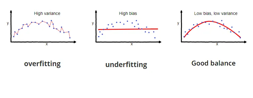
A big part of building the best models in machine learning deals with the bias-variance tradeoff. Bias refers to how correct (or incorrect) the model is. A very simple model that makes a lot of mistakes is said to have high bias. A very complicated model that does well on its training data is said to have low bias. Negatively correlated with bias is the variance of a model, which describes how much a prediction could potentially vary if one of the predictors changes slightly. In the simple model mentioned above, the simplicity of the model makes its predictions change slowly with predictor value, so it has low variance. On the other hand, our complicated, low bias model likely fits the training data very well and so predictions vary wildly as predictor values change slightly. This means this model has high variance, and it will not generalize to new/unseen data well.

The low-bias/high-variance model exhibits what is called overfitting, in which the model has too many terms and explains random noise in the data on top of the overall trend. This causes it to perform poorly on data the model has not seen before. The high-bias/low-variance model exhibits what is called underfitting, in which the model is too simple/has too few terms to properly describe the trend seen in the data. Again, the model will struggle on new data. Neither of these model types is ideal, we would like to reach some middle ground where we have the proper number of terms to describe the trend without fitting to the noise. We therefore need some sort of feature selection in which predictors with no relationship with the dependent variable are not influential in the final model.

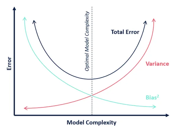
The bias-variance tradeoff is visualized above. The total error of the model is composed of three terms: the (bias)², the variance, and an irreducible error term. As we can see in the graph, our optimal solution in which total error is minimized is at some intermediate model complexity, where neither bias nor variance is high.

Weaknesses of OLS Linear Regression

Linear regression finds the coefficient values that maximize R²/minimize RSS. But this may not be the best model, and will give a coefficient for each predictor provided. This includes terms with little predictive power. This results in a high-variance, low bias model. We therefore have the potential to improve our model by trading some of that variance with bias to reduce our overall error. This trade comes in the form of regularization, in which we modify our cost function to restrict the values of our coefficients. This allows us to trade our excessive variance for some bias, potentially reducing our overall error.

Lasso

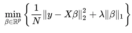
Lasso (sometimes stylized as LASSO or lasso) adds an additional term to the cost function, adding the sum of the coefficient values (the L-1 norm) multiplied by a constant lambda. This additional term penalizes the model for having coefficients that do not explain a sufficient amount of variance in the data. It also has a tendency to set the coefficients of the bad predictors mentioned above 0. This makes Lasso useful in feature selection.

Lasso however struggles with some types of data. If the number of predictors (p) is greater than the number of observations (n), Lasso will pick at most n predictors as non-zero, even if all predictors are relevant. Lasso will also struggle with colinear features (they’re related/correlated strongly), in which it will select only one predictor to represent the full suite of correlated predictors. This selection will also be done in a random way, which is bad for reproducibility and interpretation.

It is important to note that if lambda=0, we effectively have no regularization and we will get the OLS solution. As lambda tends to infinity, the coefficients will tend towards 0 and the model will be just a constant function.

Ridge Regression

Ridge regression also adds an additional term to the cost function, but instead sums the squares of coefficient values (the L-2 norm) and multiplies it by some constant lambda. Compared to Lasso, this regularization term will decrease the values of coefficients, but is unable to force a coefficient to exactly 0. This makes ridge regression’s use limited with regards to feature selection. However, when p > n, it is capable of selecting more than n relevant predictors if necessary unlike Lasso. It will also select groups of colinear features, which its inventors dubbed the ‘grouping effect.’

Much like with Lasso, we can vary lambda to get models with different levels of regularization with lambda=0 corresponding to OLS and lambda approaching infinity corresponding to a constant function.

Interestingly, analysis of both Lasso and Ridge regression has shown that neither technique is consistently better than the other; one must try both methods to determine which to use (Hou, Hastie, 2005).

Elastic Net

Elastic Net includes both L-1 and L-2 norm regularization terms. This gives us the benefits of both Lasso and Ridge regression. It has been found to have predictive power better than Lasso, while still performing feature selection. We therefore get the best of both worlds, performing feature selection of Lasso with the feature-group selection of Ridge.

Elastic Net comes with the additional overhead of determining the two lambda values for optimal solutions.