Supervised Learning - Prediction Week 3 Challenge
Prediction Week 3 Challenge
- Perform Gradient Descent in Python with any loss function.
It is an iterative first-order optimisation algorithm used to find a local minimum of a given function,until the function is close to or equal to zero, the model will continue to adjust its parameters to yield the smallest possible error. This method is commonly used in machine learning and deep learning to minimise a cost/loss function in a linear regression.
The starting point is just an arbitrary point for us to evaluate the performance. From that starting point, we will find the derivative (or slope), and from there, we can use a tangent line to observe the steepness of the slope. The slope will inform the updates to the parameters—i.e. the weights and bias. The slope at the starting point will be steeper, but as new parameters are generated, the steepness should gradually reduce until it reaches the lowest point on the curve, known as the point of convergence.
Similar to finding the line of best fit in linear regression, the goal of gradient descent is to minimize the cost function, or the error between predicted and actual y. In order to do this, it requires two data points—a direction and a learning rate. These factors determine the partial derivative calculations of future iterations, allowing it to gradually arrive at the local or global minimum (i.e. point of convergence).
- Learning rate (also referred to as step size or the alpha) is the size of the steps that are taken to reach the minimum. This is typically a small value, and it is evaluated and updated based on the behavior of the cost function. High learning rates result in larger steps but risks overshooting the minimum. Conversely, a low learning rate has small step sizes. While it has the advantage of more precision, the number of iterations compromises overall efficiency as this takes more time and computations to reach the minimum.
- The cost (or loss) function measures the difference, or error, between actual y and predicted y at its current position. This improves the machine learning model's efficacy by providing feedback to the model so that it can adjust the parameters to minimize the error and find the local or global minimum. It continuously iterates, moving along the direction of steepest descent (or the negative gradient) until the cost function is close to or at zero. At this point, the model will stop learning. Additionally, while the terms, cost function and loss function, are considered synonymous, there is a slight difference between them. It’s worth noting that a loss function refers to the error of one training example, while a cost function calculates the average error across an entire training set.
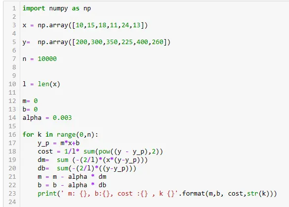
Attached the python file below, from the data set the best fit line with the minimum cost is 180.86 and corresponding m is 14.4 and b is 69.1 with learing rate 0.003 reached with iteration 6676 after this value of the cost funtion remains same.
2. Difference between L1 & L2 Gradient descent method.
Mean Absolute Error (L1) :
Mean Absolute Error(MAE) is the mean size of the mistakes in collected predictions. We know that an error basically is the absolute difference between the actual values and the values that are predicted. The absolute difference means that if the result has a negative sign, it is ignored.
Hence, MAE = Actual values – Predicted values
MAE = (1/n) * Σ|actual – Predicted |
MAE takes the average of this error from every sample in a dataset and gives the output.
Mean Squared Error (L2):
The Mean Absolute Error is the squared mean of the difference between the actual values and predictable values.
Lesser the MSE => Smaller is the error => Better the estimator.
The Mean Squared Error is calculated as:
MSE = (1/n) * Σ(actual – Predicted )2
| L1 Regularization | L2 Regularization |
| Sum of absolute value of weights | Sum of squares of wieghts. |
| Sparse solution is the outcome | Non sparse solution |
| Multiple solution are possible | Only one soution in possible |
| Robust to outliers | Not so robust to outlier due to square term |
| Used in dataset with sparse features | Used in data set with complex features |
3.What are the different loss functions for regression.
The loss functions are a measure of a machine learning model’s accuracy in predicting the predicted outcome. The cost function and loss function both relate to the same thing: the training process that employs backpropagation to reduce the difference between the actual and anticipated outcome A loss function measures how well a given machine learning model fits the specific data set. if predictions of model are perfect then loss would be very less otherwise the loss would be greater. Regardless of the problem statement, there should always be performance evaluation for comparing the predicted values with the actual values, aim would be to minimize the cost function.
Different loss function are
- Mean Absolute Error
- Mean Squared Error
- Root Mean Squared Error
- Huber Loss
- Log-loss
- Quantile Loss
Mean Absolute Error :
Mean Absolute Error(MAE) is the mean size of the mistakes in collected predictions. We know that an error basically is the absolute difference between the actual values and the values that are predicted. The absolute difference means that if the result has a negative sign, it is ignored. Even for small error there is a drastic change in slope of the regression line.
Hence, MAE = Actual values – Predicted values
MAE = (1/n) * Σ|actual – Predicted |
MAE takes the average of this error from every sample in a dataset and gives the output.
Mean Squared Error :
The Mean Absolute Error is the squared mean of the difference between the actual values and predictable values. Magnifies errors and disturbs loss funtions in case of outliers.
Lesser the MSE => Smaller is the error => Better the estimator.
The Mean Squared Error is calculated as:
MSE = (1/n) * Σ(actual – Predicted )2
Root Mean Squared Error:
Root Mean Squared Error is the square root of Mean square error. As we are applying square root to MSE, RMSE comes down to the same unit as the target variable. The loss function of RMSE is exactly the same as MSE, we just brought down the order from 2 to 1 so that correlation can be easily done. The correlation becomes difficult in MSE because it severely penalizes large errors.
RMSE = √( (1/n) * Σ(actual – Predicted )2)
Huber Loss:
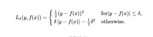
Huber Loss combines the robustness of L1 with the stability of L2, essentially the best of L1 and L2 losses. For huge errors, it is linear and for small errors, it is quadratic in nature. Huber loss approaches MSE for small error and approaches MAE in case of outliers.
Log Loss:
Logarithmic loss indicates how close a prediction probability comes to the actual/corresponding true value.Log Loss is the most important classification metric based on probabilities. It’s hard to interpret raw log-loss values, but log-loss is still a good metric for comparing models. For any given problem, a lower log loss value means better predictions.

Quantile Loss:
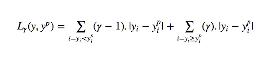
A quantile is a value below which a fraction of samples in a group falls. Machine learning models work by minimizing (or maximizing) an objective function. As the name suggests, we apply the quantile regression loss function to predict quantiles. For a set of predictions, the loss will be its average.Quantile loss function turns out to be useful when we’re interested in predicting an interval instead of only point predictions.
4.What is the importance of learning rate.
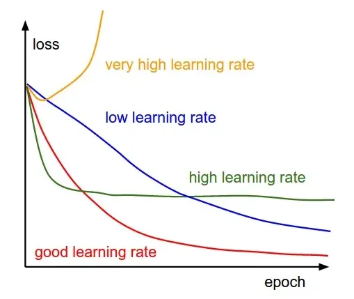
In machine learning, the learning rate is a hyperparameter that controls how much to update the model in response to the estimated error each time the model weights are updated. It determines the step size at each iteration while moving toward a minimum of a loss function. A learning rate that is too small can result in a slow convergence, while a learning rate that is too large can result in overshooting the minimum of the loss function. Finding an appropriate learning rate is crucial for the success of a machine learning model.Learning rate (λ) is one such hyper- parameter that defines the adjustment in the weights of our network with respect to the loss gradient descent. It determines how fast or slow we will move towards the optimal weights.
- Both low and high learning rates results in wasted time and resources
- A lower learning rate means more training time.
- More time results in increased cloud GPU costs
- A higher rate could result in a model that might not be able to predict anything accurately.
5.How to evaluate linear regression
Linear regression models can be evaluated using various metrics, some of which are:
- Mean Squared Error
- Root Mean Squared Error
- R-squared
- Adjusted R-squared
- Mean Absolute Error
- Residual plot
-
Mean Squared Error (MSE): It is the average of the squared differences between the predicted and actual values. A lower MSE indicates better model performance.
-
Root Mean Squared Error (RMSE): It is the square root of the MSE. It provides an estimate of the standard deviation of the residuals. A lower RMSE indicates better model performance.
-
R-squared (R²): It measures the proportion of variance in the dependent variable that is explained by the independent variable(s). R² values range from 0 to 1, with higher values indicating a better fit.
-
Adjusted R-squared (R²adj): It adjusts the R² value for the number of independent variables used in the model. It penalizes the inclusion of irrelevant independent variables.
-
Mean Absolute Error (MAE): It is the average of the absolute differences between the predicted and actual values. A lower MAE indicates better model performance.
-
Residual plot: It is a plot of the residuals (difference between the predicted and actual values) against the independent variable(s) used in the model. A random scatter of points around zero indicates a good fit, while a pattern in the plot indicates a poor fit.
6.What is the difference between multiple and adjusted coefficient of determination.
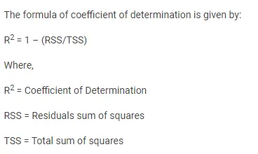
The coefficient of determination:The coefficient of determination, R2, is used to analyze how differences in one variable can be explained by a difference in a second variable R-squared gives you the percentage variation in y explained by x-variables. The range is 0 to 1 (i.e. 0% to 100% of the variation in y can be explained by the x-variables).
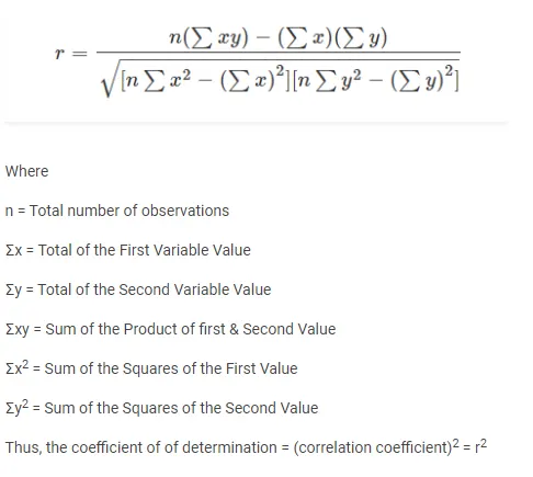
The coefficient of determination or R squared method is the proportion of the variance in the dependent variable that is predicted from the independent variable. It indicates the level of variation in the given data set.
The coefficient of determination is the square of the correlation(r), thus it ranges from 0 to 1.
With linear regression, the coefficient of determination is equal to the square of the correlation between the x and y variables.
- If R2 is equal to 0, then the dependent variable cannot be predicted from the independent variable.
- If R2 is equal to 1, then the dependent variable can be predicted from the independent variable without any error.
- If R2 is between 0 and 1, then it indicates the extent that the dependent variable can be predictable. If R2 of 0.10 means, it is 10 percent of the variance in the y variable is predicted from the x variable. If 0.20 means, 20 percent of the variance in the y variable is predicted from the x variable, and so on.
The value of R2 shows whether the model would be a good fit for the given data set. In the context of analysis, for any given per cent of the variation, it(good fit) would be different. For instance, in a few fields like rocket science, R2 is expected to be nearer to 100 %. But R2 = 0(minimum theoretical value), which might not be true as R2 is always greater than 0( by Linear Regression).
Adjusted coefficient of determination:
The Adjusted Coefficient of Determination (Adjusted R-squared) is an adjustment for the Coefficient of Determination that takes into account the number of variables in a data set. It also penalizes you for points that don’t fit the model.Basically calculate R square from only those variables whose addition in the model which are significant .Adjusted coefficient of determination is the adjusted value of the coefficient of determination in which the number of variables of the data set is taken into consideration. It determines the fitting of the multiple regression equations for the sample data. It is also known as adjusted or . It determines the proportion of variation which is determined by the estimated line of regression.
The adjusted coefficient of determination takes the values between 0 and 1. It explains the percentage of variation of the independent variables that affect the dependent variables. If the adjusted coefficient of determination is closer to 1, it indicates that the estimated equation of regression fits the data. The value of the adjusted coefficient of determination increases only when new independent variables are added which in turn increases the power of the regression equation. Hence, adjusted coefficient of determination is widely used in multiple regression analysis. In this way, it is very useful measure than the coefficient of determination.The adjusted coefficient of determination is always less than or equal to the coefficient of determination. The addition of independent variables that do not fit the model will be penalized by the adjusted coefficient of determination. If the adjusted coefficient of determination is negative, it indicates that the model does not fit the data.
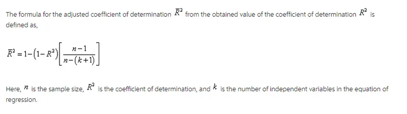
The most vital difference between adjusted R-squared and R-squared is simply that adjusted R-squared considers and tests different independent variables against the model and R-squared does not.