Steady Vs Unsteady flow over a cylinder
➤OBJECTIVE : To simulate the flow over a cylinder using steady and unsteady state solvers and explain the phenomenon of karman vortex street.
◙ PART I : (1) Simulate the flow with the steady and unsteady case and calculate the Strouhal Number for Re=100.
◙ PART II : (1) Calculate the coefficient of drag and lift over a cylinder by setting the Reynolds number to 10,100,1000,10000 & 100000. (Run with steady solver)
(2) Discuss the effect of Reynolds number on the coefficient of drag.
➤ Introduction of Karman Vortex Effect:
In fluid dynamics, vortex shedding is an oscillating flow that takes place when a fluid such as air or water flows past a bluff (as opposed to streamlined) body at certain velocities, depending on the size and shape of the body. In this flow, vortices are created at the back of the body and detach periodically from either side of the body forming a Von Karman vortex street which is responsible for the unsteady separation of the flow of a fluid around blunt bodies. It is named after the engineer and fluid dynamicist Theodore von karman. The fluid flow past the object creates alternating low-pressure vortices on the downstream side of the object. The object will tend to move toward the low-pressure zone.
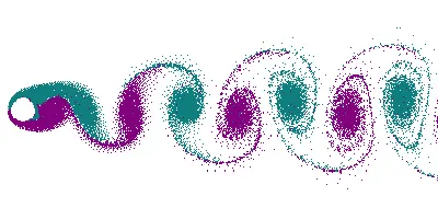
Animation of vortex street created by a cylindrical object; the flow on opposite sides of the object is given different colors, showing that the vortices are shed from alternating sides of the object.
➤ Physics behind vortex formation:
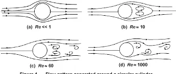
Flow patterns generated around a circular cylinder immersed in a uniform flow are shown in above figure. The pattern of this flow varies depending upon the Reynolds number. Figure 1-(a) shows a flow with a very small Reynolds number. The shape of every streamline is symmetrical not only around the cylinder’s upper to lower side, but also around its front to rear. As the Reynolds number increases, the front to rear symmetry disappears, and the interval of the streamlines of the cylinder’s rear flow widens. As the Reynolds number reaches close to 10, a closed region of the streamline is generated within the cylinder’s rear flow. The fluid in the upper half of this region rotates clockwise, and the fluid in the lower half rotates counter clockwise. This phenomenon is the result of the so-called generation of vortices. Figure 1-(b) depicts this state.
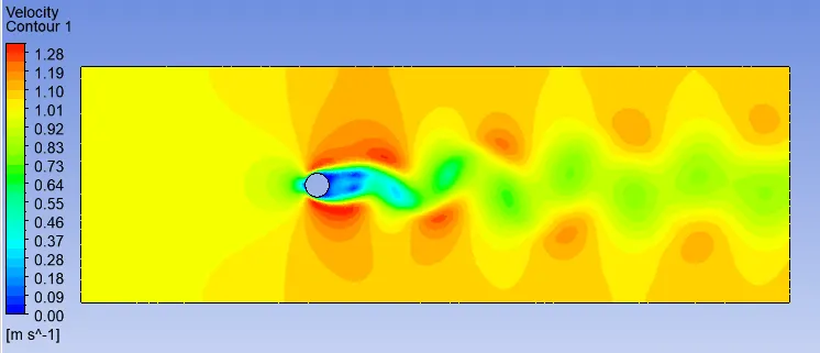
As the Reynolds number increases, the length of the vortex increases. When the Reynolds number exceeds 60, the rear flow becomes unstable as shown in Figure 1-(c), and the vortex begins to oscillate in an up-down direction. The fully formed vortex is carried away on the surrounding main flow, and a vortex subsequently occurs on the other side. This vortex then expands before finally dissipating and departing leaving the circular cylinder. In addition to this flow process, every pair of upper and lower vortices behind the cylinder is stored in an alternative regular array to form twin rows of vortices. These rows are called the von Karman vortex street. While the main flow approaching the circular cylinder is in a uniformly steady state, a periodically varying flow characteristic of the von Karman vortex street appears in the cylinder’s rear flow.
As shown in Figure 1-(d), as the Reynolds number reaches 1,000, the vortices are mixed together, and the flow behind the cylinder (wake) behaves very irregularly in time and space scale. This behavior is the so-called state of turbulent flow. However, a free stream distant from the wake region maintains a steady state, and the streamlines are held in a regular and smooth shape. This phenomenon is known as laminar flow.
➤ Importance of Karman Vortex street:
The Karman street can lead to unwanted noise or even cause failure of structures when the vortexshedding frequency coincides with the natural frequency of structure. This type of vortex-inducedoscillations can occur in a variety of situations such as chimneys, bridges, heat exchanger tubes,overhead power cables and marine structures. Therefore understanding the physics of the Karmanvortex street is crucial to avoid disasters in these situations.
➤ PROCEDURE :
(1) Geometry Creation :
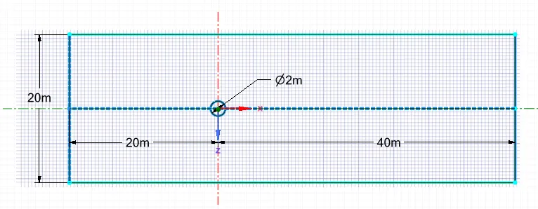
➦ Computational Domain :
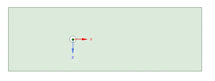
➦ 2D Geometry :
Sketch the 2D cylinder of diameter 2 meter by following the above standard dimesions. Then do the surface generation in spaceclaim by deleting the inside circle in order to carry out the simulation.
(2) Mesh Generation :
★ Method : By default, Ansys meshing creates a quadrilateral dominant mesh. We need to convert it into Triangles.
Go to Mesh → Insert → Method → Select face → Method(Triangles) → Generate Mesh
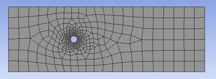
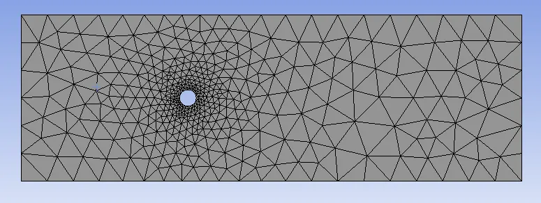
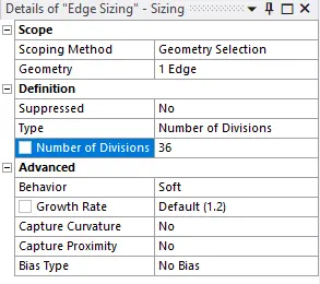
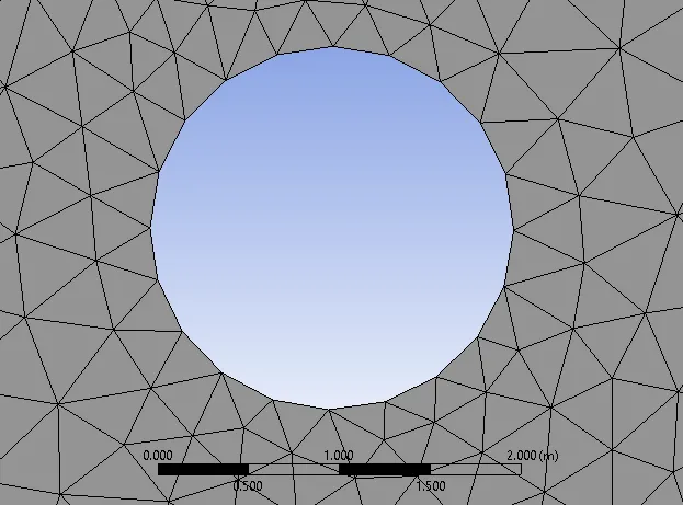
★ Sizing : The cylinder we have is not perfectly circular, these sharp corners may effects the flow field. so if we proceed like that geometry there might be inaccuracy in results. This option will help us to create smooth curves by dividing the circle into large numbers of edges.
Go to Sizing → Select Edge → Type (Number of divisions) → Enter number and Generate Mesh
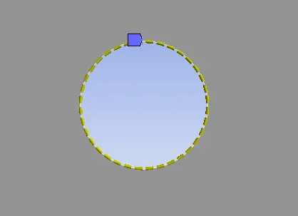
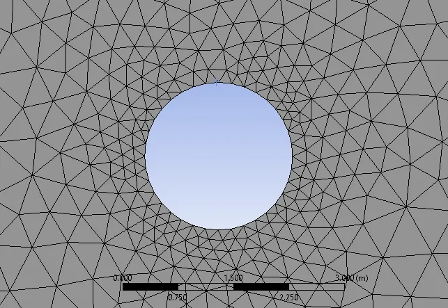
★ Inflation : Since the flow around the cylinder is important, so we need to resolve the boundary over the cylinder for that we require finer mesh around the cylinder. So in that aspect Inflation layer helps us to create ' Body fitted Mesh ' over the region around the cylinder.
Go to Inflation → Select Face → Select Edge → Number of layers → Enter number and Generate Mesh
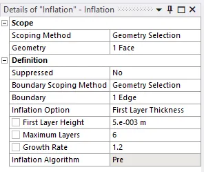
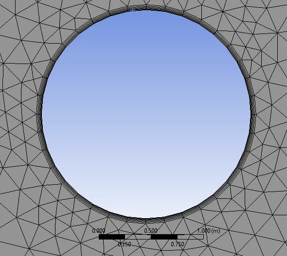
★ Final Mesh : Here, for all case studies, we will be using a 0.25m mesh size.
◙ PART I :
➦ Reynolds Number(Re) :
A vortex street will form only at a certain range of flow velocities, specified by a range of Reynolds numbers(Re), typically above a limiting Re value of about 90. The Reynolds number for a flow is a measure of the ratio of inertial to viscous forces in the flow of a fluid around a body or in a channel.
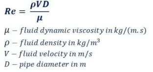
➦ Vary the velocity of the flow to change the Reynolds number.
Material : user-defined material with following properties (density = 1 kg/m3 and dynamic viscosity = 0.02 kg/m.s)
For Re = 100 :
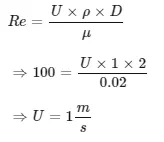
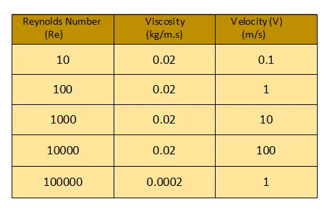
Table : velocities for corresponding Reynolds numbers.
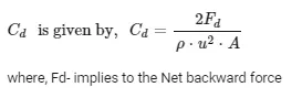
➦ Coefficient of Drag :
The aerodynamic drag coefficient is a measure of the effectiveness of a streamline aerodynamic body shape in reducing the air resistance to the forward motion of a vehicle. A low drag coefficient implies that the streamline shape of the vehicle's body is such as to enable it to move easily through the surrounding viscous air with the minimum of resistance; conversely, a high drag coefficient is caused by poor streamlining of the body profile so that there is a high air resistance when the vehicle is in motion.
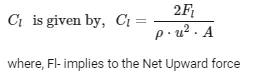
➦ Coefficient of Lift :
The lift coefficient (CL) is a dimensionless coefficient that relates the lift generated by a lifting body to the fluid density around the body, the fluid velocity, and an associated reference area.
(3) Fluent Setup :
★ First run Perform Check mesh in order to find any kind of errors in the geometry.
★ Physics :
→ Solver : Pressure Based.
→ Viscous model : Laminar.
→ Material : user-defined material with following properties (density = 1 kg/m3 and dynamic viscosity = 0.02 kg/m.s).
★ Boundary Conditions :
→ Inlet : Velocity Inlet
Velocity Magnitude- 1 m/s
→ Outlet : Pressure outlet
Gauge Pressure- 0 Pa
→ Symmetry : Symmetry
Zone name- Symmetry
→ Walls : Wall
Wall motion- Stationary wall
Shear condition- No slip
★ Solving :
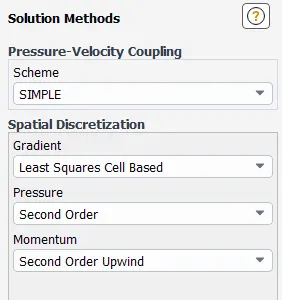
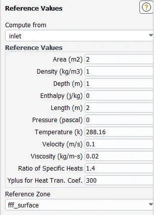
Here, Area = Height*Width =2 m2.
Height = 2m.
Width = 1m because analysis in 2D.
For all 2D problems Depth =1m.
Length = 2m (because here length means flow length along the direction of flow which is the diameter = 2m).
★ Solutions :
➦ Create a Vertex average of velocity magnitude using surface report at a monitor point 8D from the center of the cylinder to the right of the cylinder along X-direction.
➦ Initialization method- Hybrid for STEADY STATE simulations
Standard for UNSTEADY STATE simulations
➦ Coefficient of Drag and Coefficient of Lift report created using force report.
➦ activities: Contour plots of Pressure & Velocity and Solution animation need to create after initializing the solution.
➦ Run calculation:
For STEADY STATE- Nos. of iterations= 500
For TRANSIENT STATE- Time_Step= 0.1
Nos. of iterations= 2000
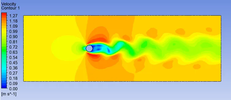
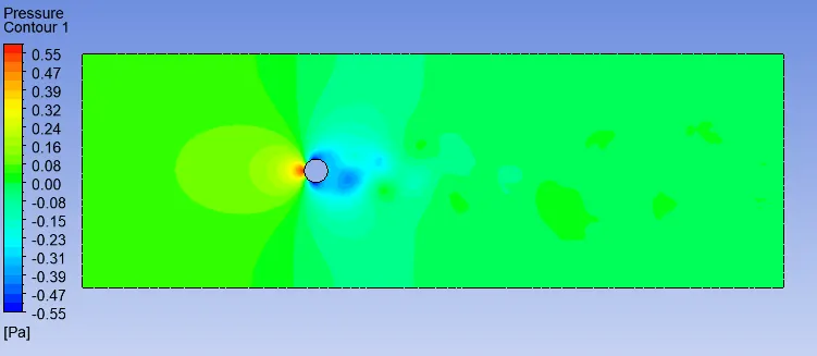
◙ In this case study flow over cylinder has been presented where Re.No. is taken as 100 and both STEADY state and TRANSIENT state simulated.
◙ Results: For STEADY STATE (Re =100)
In steady-state, nos. of iteration is 500 and viscosity 0.02 kg/m-s for Re. no.100.
◘ Residual or Convergence plot: The role of this residual plot is to monitor the change in each and every convergence criterion for every time step and plot those values for every iteration or timestep. This plot helps us in knowing at what point convergence is achieved.
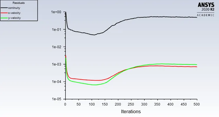
From the above graph, we can see, the solution has reached a steady-state even much before 500 iterations.
◘ Coefficient of drag(Cd) & Coefficient of lift(Cl)plots:
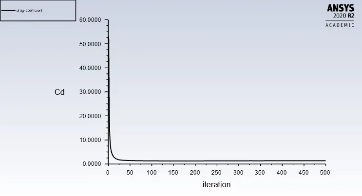
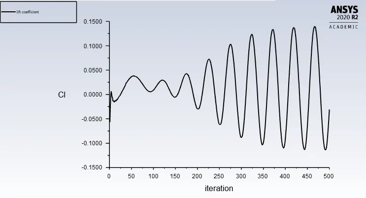
The values for Cd and Cl are found out 1.3358462 and -0.030817293 respectively.
◘ Monitor point velocity plot : A monitor point is placed at a distance of 8m from the cylinder inorder to calclate the velocity at that point.
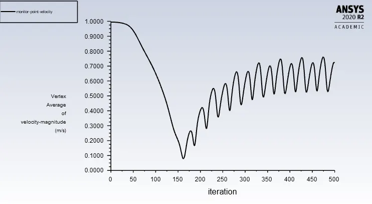
The value for the Vertex average of velocity magnitude at the monitoring point is 0.722381 m/s.
◘ Velocity Contour plot : (Showing Vortex Shedding Effect)
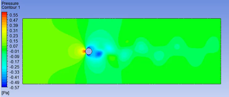
◘ Pressure Contour plot : (For visualizing the magnitude of pressure difference at up and downstream side of the cylinder).
◙ Results: For TRANSIENT STATE (Re =100)
In the Transient case, we will be stimulating with Timestep of 0.1 sec for 2000 iterations.viscosity 0.02 kg/m-s for Re. no.100.
◘ Residual or Convergence plot:
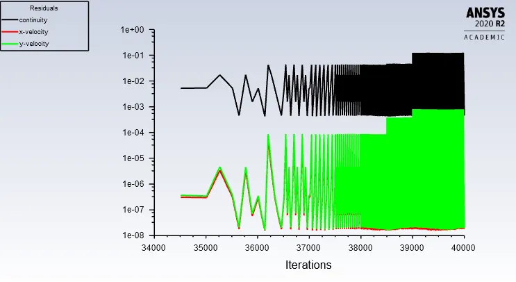
Since we are looking for time-based vortex formation that is why we can see lots of Fluctuations in the convergence plot.
◘ Coefficient of drag(Cd) & Coefficient of lift(Cl)plots:
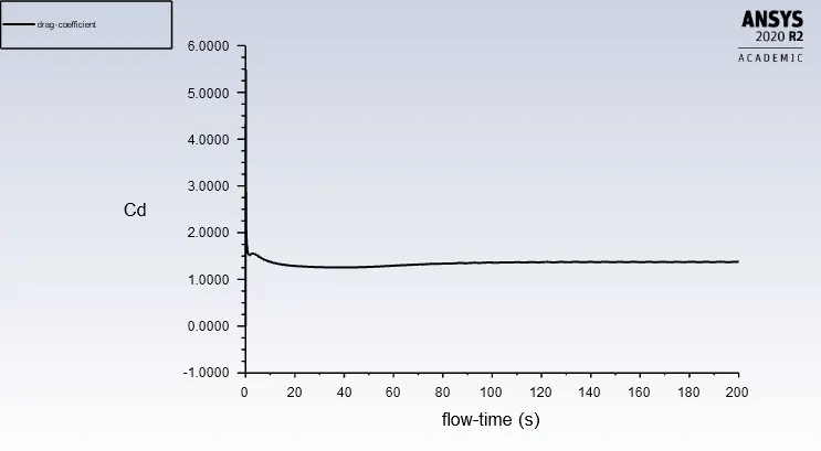
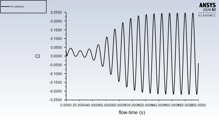
The values for Cd and Cl are found out 1.3713954 and -0.039919702 respectively.
◘ Monitor point velocity plot :
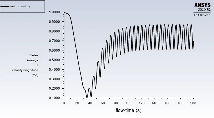
The value for the Vertex average of velocity magnitude at the monitoring point is 0.6969676 m/s.
◘ Velocity Contour plot :
◘ Pressure Contour plot :
★ Strouhal Number:
The Strouhal Number is a dimensionless value useful for analyzing oscillating unsteady fluid flow dynamics problems.
The Strouhal Number can be important when analyzing unsteady, oscillating flow problems. The Strouhal Number represents a measure of the ratio of the inertial forces due to the unsteadiness of the flow or local acceleration to the inertial forces due to changes in velocity from one point to an other in the flow field.
Thus, an alternative definition of the Strouhal number better suited to periodic flows is given by the following expression:

Where f - Frequency of vortex shedding/ oscillations
L - characteristic length
U - flow velocity
➦ For Steady State :
Strouhal number cannot be calculated for the steady state as there is no time parameter which is required in frequency calculation and can only be calculated for unsteady state condition.
➦ For Transient State :
f=No.of peaks/Flow time = 2/20 = 0.1Hz
f=0.1Hz
St = (0.1 * 2)/ 1 = 0.2
Therefore, Strouhal Number (St) = 0.2
From standard literature available on vortex shedding, it is stated that at Strouhal number values of 0.2-0.3, the vortex shedding can be observed. Also the Strouhal number also varies with Reynold's number.
◙ PART II : (1) Steady State simulation
➦ In this part, we will be calculating the Coefficient of drag and coefficient of lift for various Re. No's.
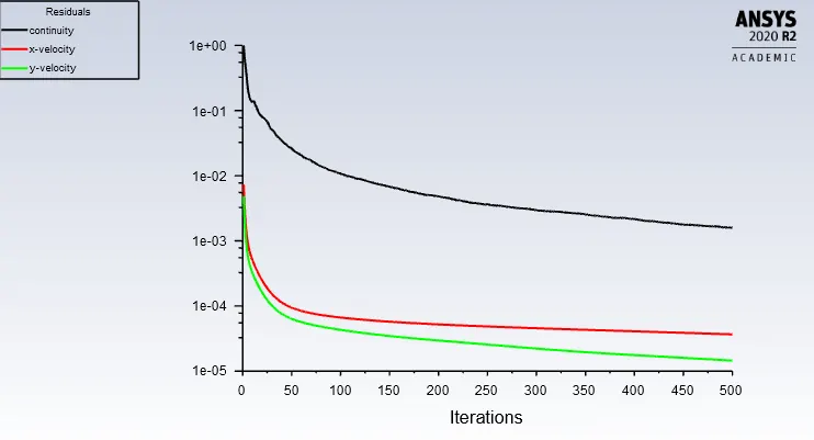
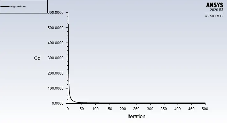
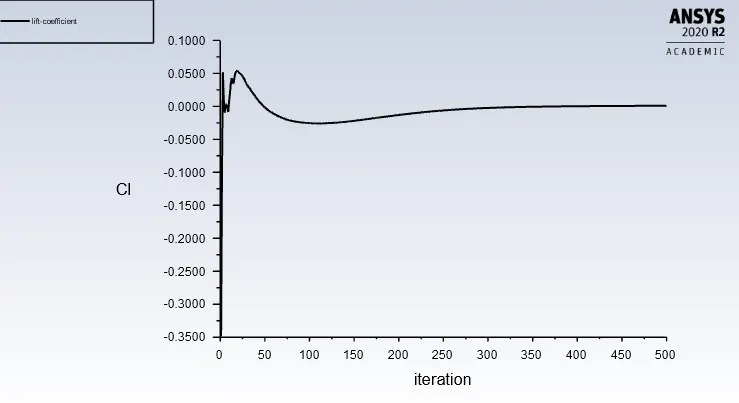
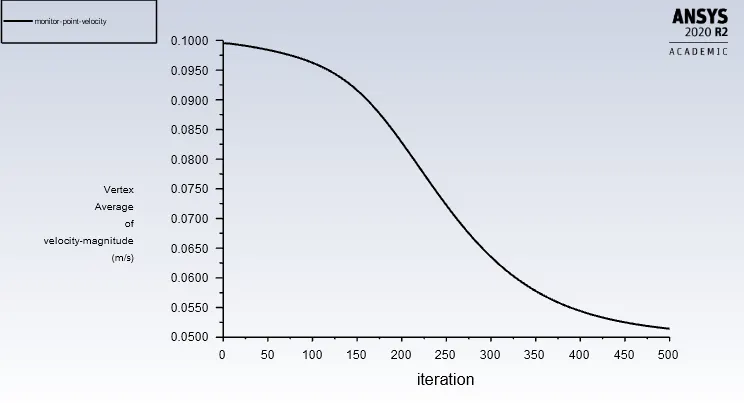
★ Case - 01 : For Re=10 where viscosity=0.02 kg/m.s and velocity=0.1m/s
◘ Residual or Convergence plot:
◘ Coefficient of drag(Cd) & Coefficient of lift(Cl)plots:
◘ Monitor point velocity plot :
◘ Velocity Contour plot :
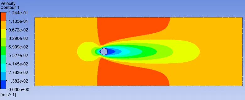
No vortex shedding is observed behind the cylinder (sphere in 2D) for Re=10.
◘ Pressure Contour plot :
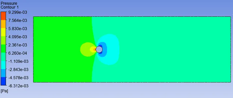
★ Case - 02 : For Re=100 where viscosity=0.02 kg/m.s and velocity=1m/s
◘ Residual or Convergence plot:
◘ Coefficient of drag(Cd) & Coefficient of lift(Cl)plots:
◘ Monitor point velocity plot :
◘ Velocity Contour plot :
◘ Pressure Contour plot :
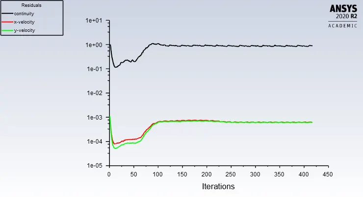
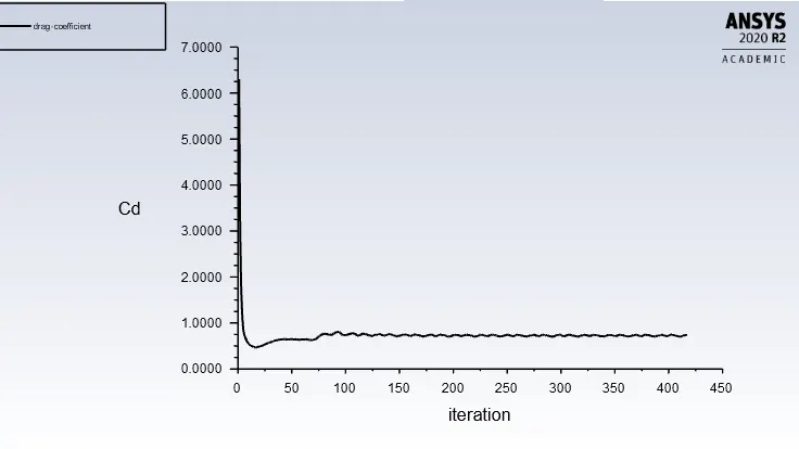
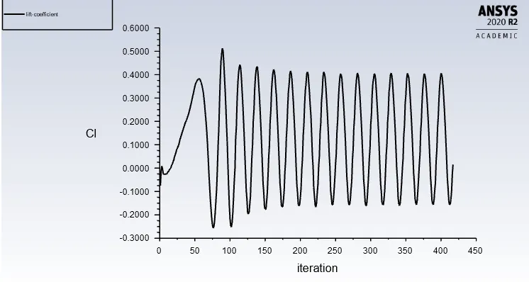
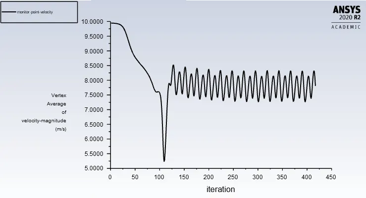
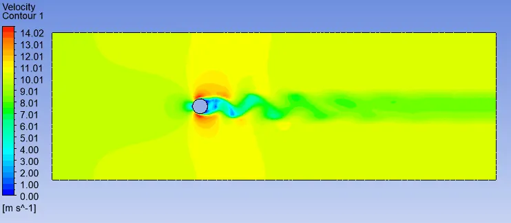
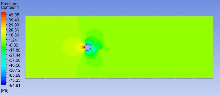
★ Case - 03 : For Re=1000 where viscosity=0.02 kg/m.s and velocity=10m/s
◘ Residual or Convergence plot:
◘ Coefficient of drag(Cd) & Coefficient of lift(Cl)plots:
◘ Monitor point velocity plot :
◘ Velocity Contour plot :
◘ Pressure Contour plot :
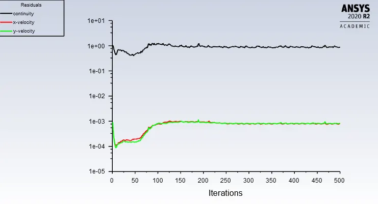
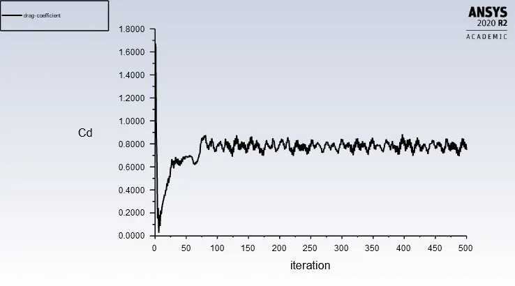
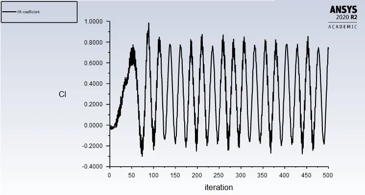
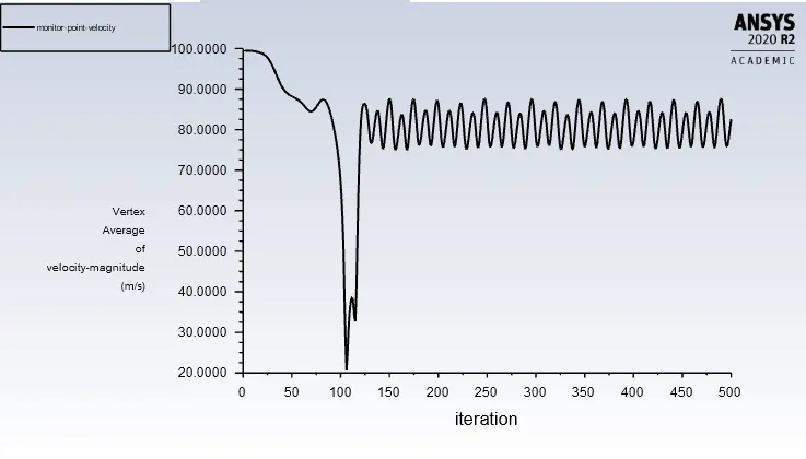
★ Case - 04 : For Re=10000 where viscosity=0.02 kg/m.s and velocity=100m/s
◘ Residual or Convergence plot:
◘ Coefficient of drag(Cd) & Coefficient of lift(Cl)plots:
◘ Monitor point velocity plot :
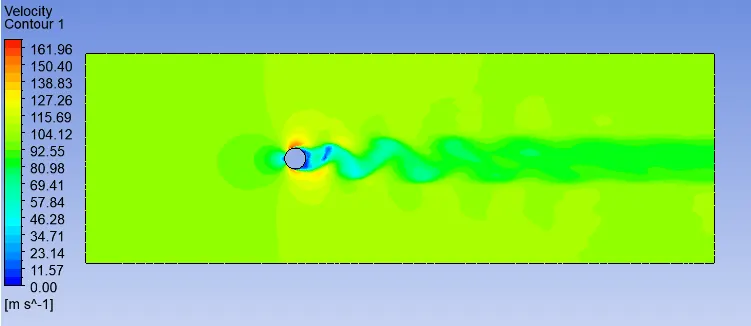
◘ Velocity Contour plot :
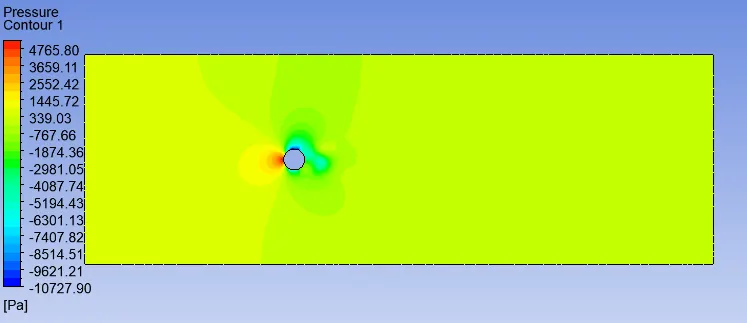
◘ Pressure Contour plot :
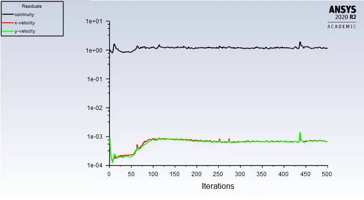
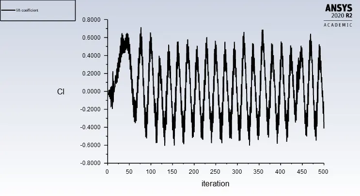
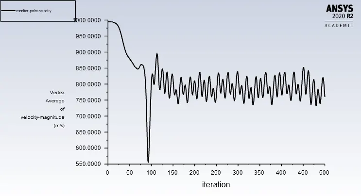
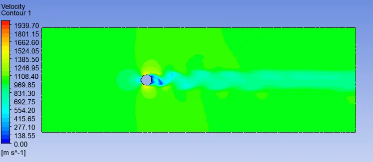
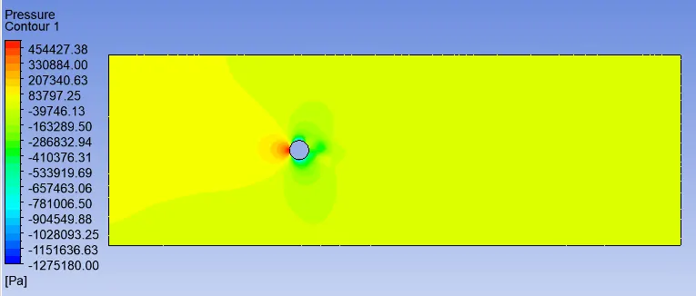
★ Case - 05 : For Re=100000 where viscosity=0.02 kg/m.s and velocity=1000m/s
◘ Residual or Convergence plot:
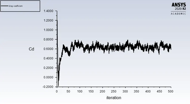
◘ Coefficient of drag(Cd) & Coefficient of lift(Cl)plots:
◘ Monitor point velocity plot :
◘ Velocity Contour plot :
◘ Pressure Contour plot :
◙ Table showing values of Cd and Cl with various Re. Nos.:
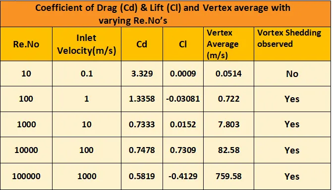
Here, in some cases we have found negative lift, it just means the force is acting downward.
(2) Effect of Reynolds Number on Drag Coefficient(Cd):
From the above table, we can observe that as reynolds number increases, drag coefficient decreases till Re = 1000 but at Re = 10000 we see a slight increase in drag coefficient and again for Re = 100000 the drag oefficient value decreases.
when the boundary layer separates and the recirculations appear, the pressure behind the cylinder (where the wakes are located) will drop, creating a drag. This is similar to what happens when vortices appear at the end of an airplane wing, the result is a drag force.
There are really two contributions to the drag force. One comes from the inertia of the fluid (the object actually collides with molecules) and the other comes from the viscosity. As Re increases, the size of the viscosity, relative to the other parameters, is decreasing. This means that the viscosity term in Navier-Stokes equation is relatively less important. Since the viscosity plays a smaller role, we would expect the contribution to drag due to viscosity to decrease.
➤ Conclusion :
★ As Reynolds Number (Re) goes increasing inertial forces starting to dominate over viscous forces. The coefficient of drag (Cd) starts decreasing and there is a significant fluctuation in the Coefficient of lift (Cl) and Vertex average of Velocity magnitude at monitoring point start rising at the same time.
★ Strouhal number was calculated for the transient condition.
★ Different reynolds number were introduced to see the vortex shedding phenomena behind the cylinder.
★ For achieving results near experimental results,Y plus value or first layer thickness is utmost important.