Ahmed Body Challenge
➤ Aim : To simulate the flow over an Ahmed body and to calulcate the values of drag and lift co-efficients generated. Also to understand flow separation, how wake forms and how it affects the flow and also to perform grid independency test.
➤ Introduction :
• The CFD (Computational Fluid Dynamics) analysis is used in the automobile industry. This analysis is used to understand the fuel consumption, stability of the vehicle and passenger comfort. It is used to analyze the Aerodyanmic flow around a common vehicle. This is an important study because the aerodynamic flow has a geater effect on the handling and overall performance of an automobile.
• The external surface of the car is very important in aerodynamics aspects of vehicles such as stability, comfort and fuel consumption at high speeds. The improvement of the aerodynamics of car shapes, more precisely the reduction of their drag coefficient, becomes one of the main topics of the automotive research sectors. Designing a vehicle with a minimized drag resistance provides economical and performance advantages. Decreased resistance to forward motion allows higher speeds for the same power output.
➤ Theory :
➥ Ahmed Body :
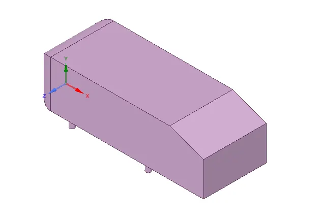
• A great deal of studies regarding airflow and turbulence behaviour on a car involve the use of the ‘Ahmed body’, which was first devised by S, Ahmed in 1984. The shape of the Ahmed body is designed in such a way to mimic the typical flow field features of a car bluff body.
• The Ahmed body is made up of a round front part, a moveable slant plane placed at back part of the body to study the coefficient of drag and separation phenomena at different angles, and a rectangular box, which connects the front part and the rear slant plane. As the wake separation flow behind the Ahmed body is the main contributor to the drag force, accurate prediction of the separation process and the wake flow are the key to the successful modelling of this case.
• Ahmed body is a generic car body (a simplified car model) i.e the flow of air around Ahmed body captures the essential flow features around an automobile.
➥ Importance of Ahmed Body :
• The air flow over ground vehicle is analysed and coefficient of drag is calculated using CFD (Ansys Fluent). For this calculation, Ahmed body (simplified car body) as ground vehicle is considered which is commonly used as test case in industry. The flow of air around Ahmed body captures the essential flow features around an automobile.
• People working in vehicle aerodynamics use Ahmed body to validate their numerical model because the experimental data from wind tunnel testing is available for Ahmed body. Once the numerical model in validated, it is used to design new models of the car.
• Drag force experienced by the car always resist the body hence decreasing the speed of car therefore main aim is to see for flow behaviour and calculate the drag force or drag coefficient, location where the flow separates is seen to get the better idea is wake region formed behind the model.
➤ PROCEDURE :
(1) Geometry Creation :
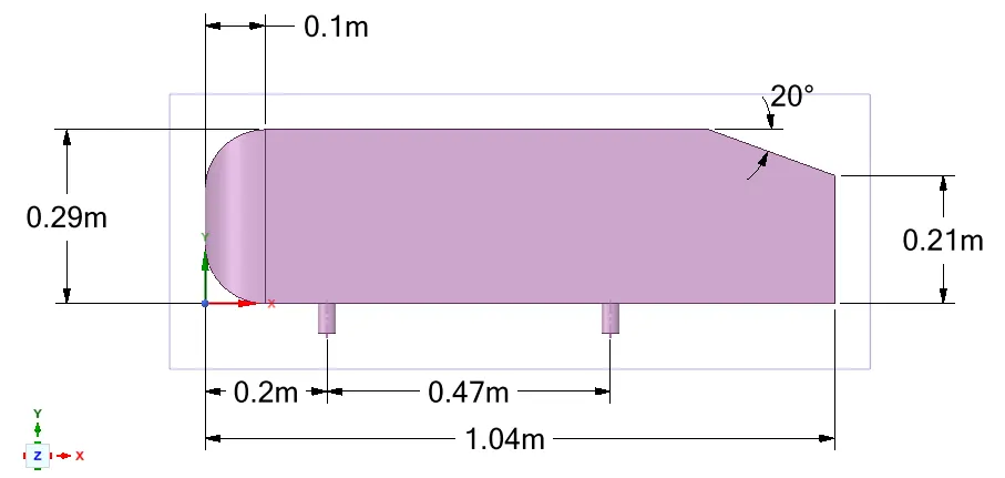
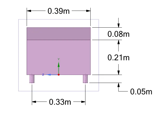
➦ Model Dimesions :
➦ Creating a Virtual Wind Tunnel :
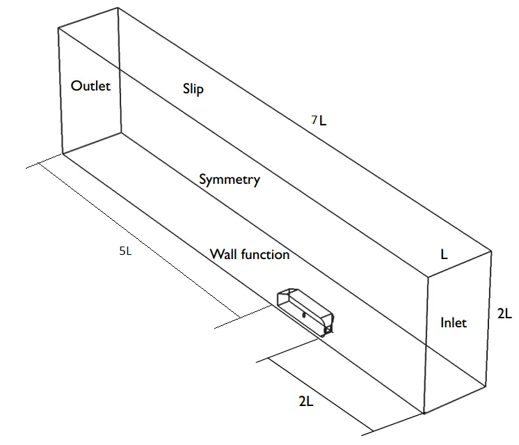
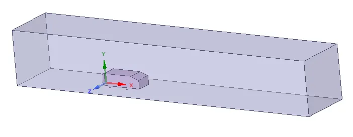
Wind tunnel is an aerodynamic facility to visualize the flow over an external surface. So in here we provide an enclosure to the ahmed body which acts as a wind tunnel. Hence setting up a good wind tunnel is a crucial point in any CFD analysis.
➦ Ahmed Body with an rectangular enclosure :
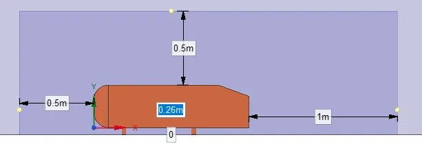
Enclosure tool is used to construct a virtual wind tunnel around the Ahmed Body.
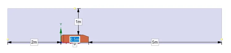
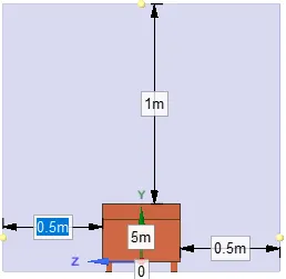
➦ Enclosure Dimensions :
➦ Simulation with Base Mesh :
Once this geometry is get prepared in Spaceclaim, it has provided with a base mesh using the meshing interface of ansys. Setup the physics and details required, then run the simulation for 100 iterations. Check the velocity contour and pressure contour plots and simulations in the fluent. Since the base line mesh is very coarse, from the velocity contour we will get a rough picture of wake region formed, so based on this one more enclosure is provided.
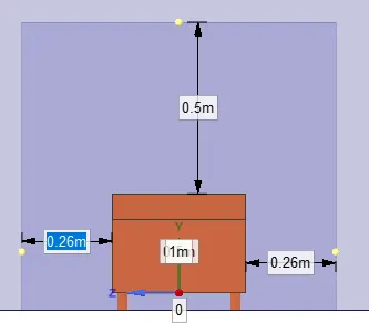
➦ Ahmed Body with an Inner enclosure :
To capture flow characteristics near the Ahmed body efficiently, local mesh refinement with a smaller element size has to be needed. For that Inner enclosure has to be created.
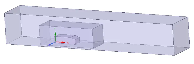
➦ Inner enclosure Dimensions :
➦ Considering Half Body :
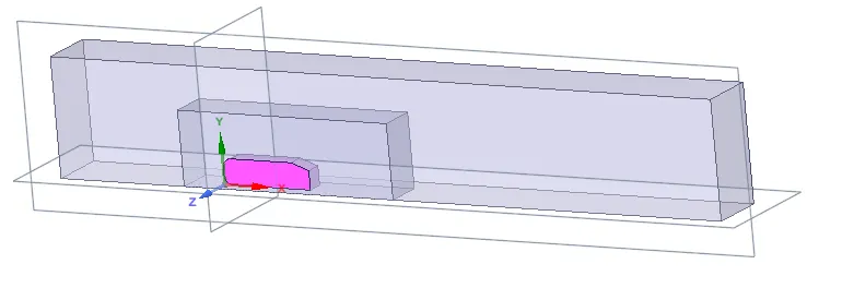
• we can mesh the above setup and it can be used for simulations, but meshing the whole setup will increase the number of cells, so as an alternative since the whole setup is completley symmetric the setup is split and share topology option is used so that information between the cells get shared. When splitted the whole setup looks like below.
• As the body is perfectly symmetric, we can simulate by considering the only half body. This is the best practice where you can save on the number of cells and get the results faster as well. Using the 'Split body' command in SpaceClaim to operate and then using the symmetry boundary condition in fluent to perform the simulation. The split tool was done along the XY plane to perfectly cut the body from the middle.
(2) Mesh Generation :
➦ Base line Mesh :
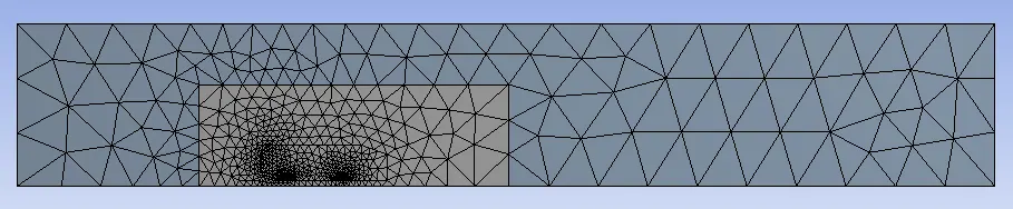
First base line mesh is added to the whole geometry, when meshed it looks as follow:
➦ Mesh modifications :
★ For the local refinement, various mesh methods were used such as Multizone, Body Sizing, Face sizing and Inflation layer.
➦ Multizone :
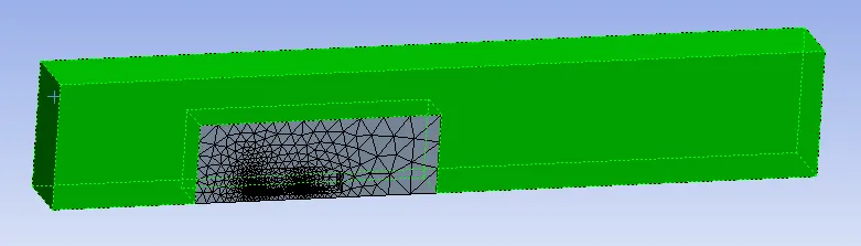
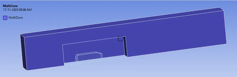
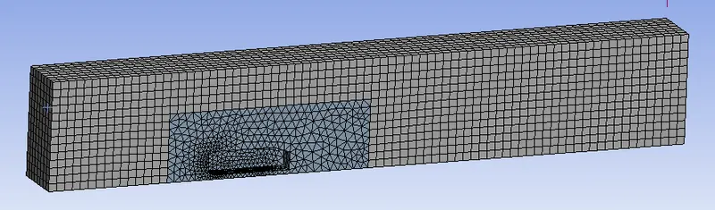
• The outer enclosure is provided with hexahedral meshes. Hexahedral meshes are the ones which are better than tetrahedral meshes, but we cannot use hexahedral meshes as such because it wont fit into complex geometries which involves curves and acute angles. When complex geometries are meshed tetrahedral can be preffered. If we observe the outer enclosure we can see that it is just a simple geometry involving only lines and hence hexahedral meshes can be used.
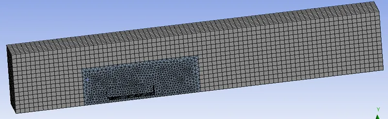
• Hexahedral meshes are added using the method option where 'Multizone' option is used to mesh the outer enclosure with hexahedral mesh. Along with adding hexahedral meshes to the enclosure the mesh element size is reduced from 419 mm (above base line mesh) to 100 mm.
• The mesh element size used for this refinement is 100 mm.

➦ Body Sizing :
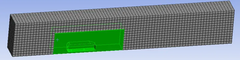
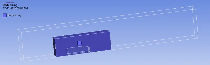
• Inner enclosure will have the typical base line tetrahedral meshes, in here the element size of the mesh is reduced using the Sizing option and hence a element size of 50 mm is used for the meshes of inner enclosure. Body sizing was used for the local area refinement around the Ahmed Body.
➦ Face Sizing :
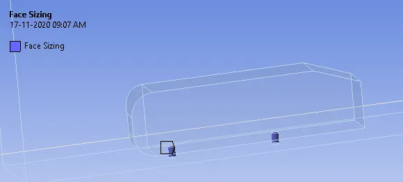
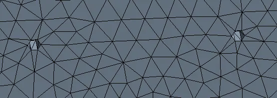
• The 2 faces of the pillar of Ahmed body which represents the tyre/wheels (for a real automobile body) was selected for face sizing. The mesh element size used was 5 mm.
➦ Inflation Layer :
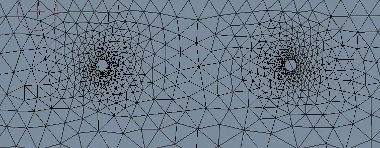
• Since we are interested in capturing wall phenomena, it will be better if we add inflation layers above ahmed body (car_wall). Inflation layers are also called as body fitted mesh, it helps in capturing gradient normal to the wall with minimum number of cells.
• The inflation layer is used to refine the local region just above the wall/body to capture the boundary layer precisely.
• While adding inflation layers one of the important aspect that is being taken care is calculation of first layer thickness. This is achieved using y+.
Before starting with first layer thickness calculation, let us start with reynolds number calculations,
★ Reynolds number, 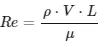
ρ - Density of fluid (kg/m^3);
V - Velocity of fluid (m/s);
L - Characteristic length of the body (m);
μ - Dynamic viscosity of fluid (kg/m*s);
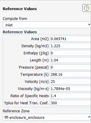
In our case we are using air as fluid, with inlet velocity , V = 25 m/s;
L = 1.04 m, which is length of ahmed body;
ρ = 1.225 kg/m^3 ;
μ = 1.7894 e -05 kg/m*s ;
therefore, Re = (1.225*25*1.04)/1.7894 e-05 = 1.77 e 06, since Re is above 2 e 05 we can consider the flow as turbulent.
Now coming to first layer thickness calculation,
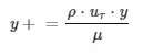
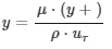
where, y is the first layer thickness.
• To understand what should be the value of y+ that we need to select so that we can calculate the value of first layer thickness and total thickness correctly, it is essential to understand the below plot,
In this simulation, y+ = 0.4 is taken and first layer thickness is calculated,
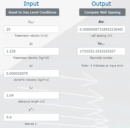
so, first layer thickness , y = 0.000005873189 m = 5.8732 e-03 mm.
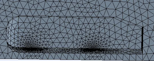
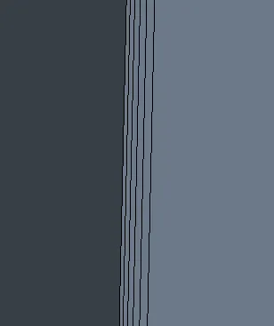
Total of 5 inflation layers are used with a growth rate of 1.2.
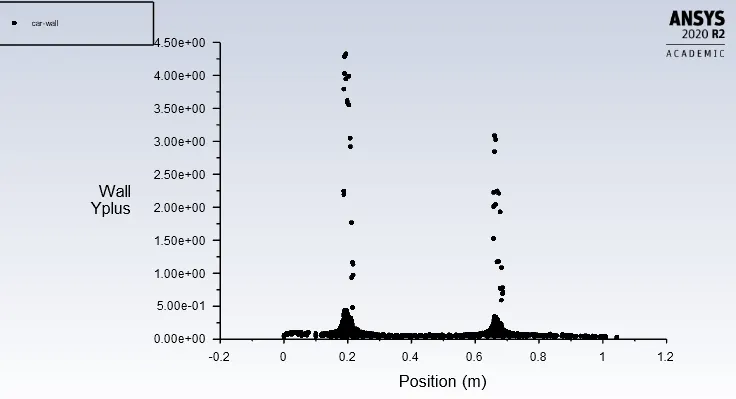
• If we were in the viscous sub-layer, that would mean a y+ of less than 10 and if we were in the turbulent region, it would mean a y+ of greater than 30. This is very significant in our making the decision of using or not using a wall function.
★ Steps for checking Y+ is in the range :
◙ Once the first layer thickness is calculated using the y+ formula, we can generate the mesh and set up the case for the first few iterations or timesteps.
◙ Once we run the simulation for a few timesteps or iteration, it is desirable to check the y+ value using the post-processing tool.
◙ The flow physics can change over the surfaces, so checking and adjusting the first layer thickness in the initial stage of the simulation is imperative to avoid remeshing and wastage of computational resources.
★ So the above value of first layer thickness is entered in the inflation options and hence we get inflation layers as shown below,
➦ Case - (01) : (" Grid size of 100 mm for outer enclosure & 50 mm for outer enclosure")
◙ Mesh metrics :
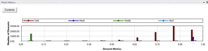
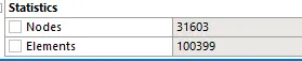
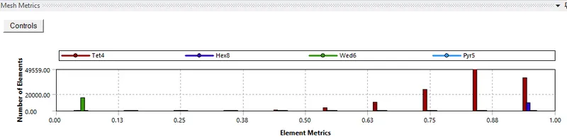
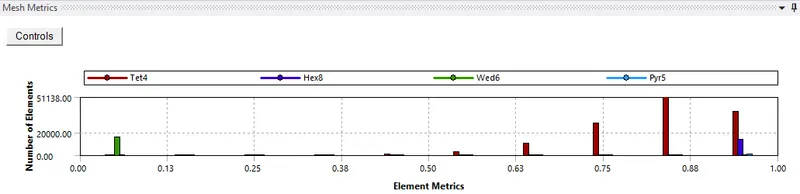
The above fig shows the proportion of tetra, hex, wedge and pyramid type of mesh incorporated under the multizone meshing type. This plot shows that we are okay to go with the minimum mesh metric criterion which is 0.38
(3) Fluent Setup :
★ First run Perform Check mesh in order to find any kind of errors in the geometry.
★ Physics :
→ Solver : Pressure Based Steady-state method opted for the simulation.
→ Viscous model : Laminar.
→ Turbulence model : ‘ k−ωSST ’
◙ This turbulence model is the combination of RNGk−ε and Standard k−ω And hence it near the wall ‘k−ωSST ’ works as a Standard k−ω model and away from the wall it works RNGk−ε model. Hence it gives an accurate prediction near the wall and away from the wall, as we are interested in capturing boundary layer growth.
◙ Also k−ωSST model is well known for it’s automatic wall-treatment, which captures boundary layer accurately. The k-ω model predicts well near the wall better.
★ Boundary Conditions :
→ Inlet : Velocity Inlet
Velocity Magnitude- 25 m/s
→ Outlet : Pressure outlet
Gauge Pressure- 0 Pa
→ Symmetry : Symmetry
Zone name- Symmetry
→ Car-Wall & Symmetry wall : Wall
Wall motion- Stationary wall
Shear condition- No slip
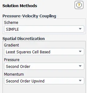
★ Solving :
◙ Results:
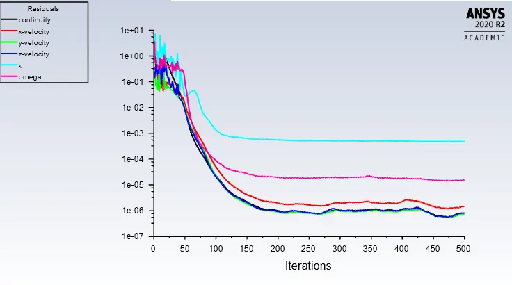
The model was initialized using Hybrid Initialization with 500 iterations to run the simulation.
◘ Residual or Convergence plot:
◘ Coefficient of drag(Cd) & Coefficient of lift(Cl) plots:
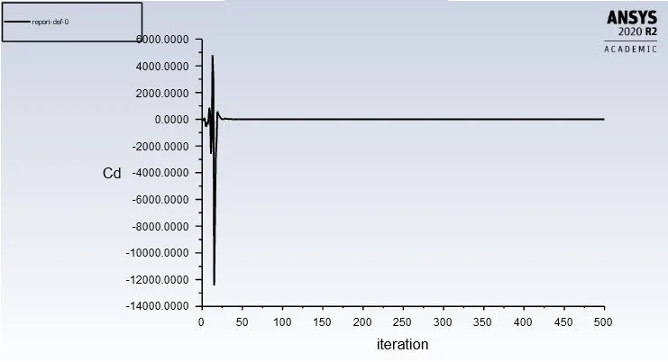
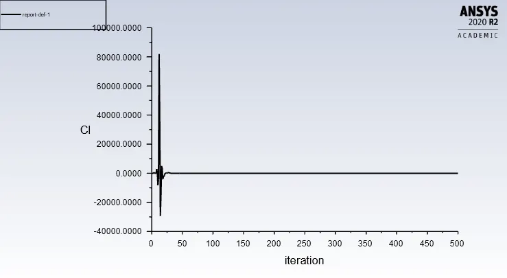
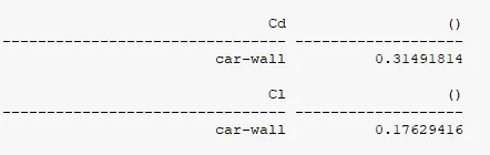
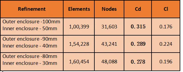
The coefficient of drag value for this mesh case comes out to be 0.3149 ≈0.315 which is much considerable as our aim was to get the value around 0.33. Similarly the coefficient of lift value comes out to be 0.1763.
◘ Velocity Contour plot :
◘ Velocity Vector plot :
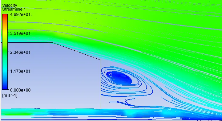
◘ Velocity Streamline plot :
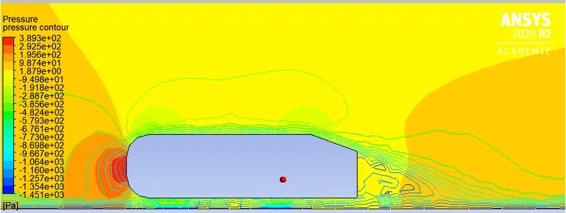
◘ Pressure Contour plot :
★ THE CONCEPT BEHIND WAKE GENERATION & NEGATIVE PRESSURE IN WAKE REGION:
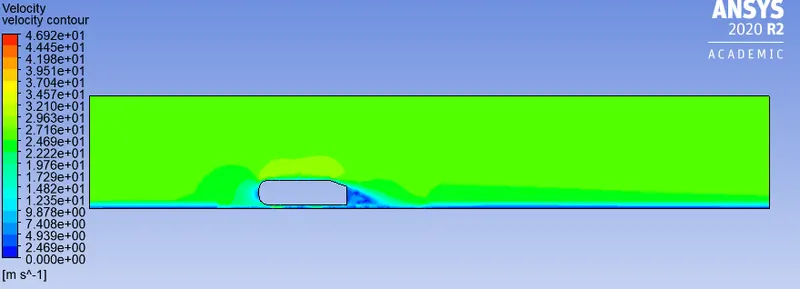
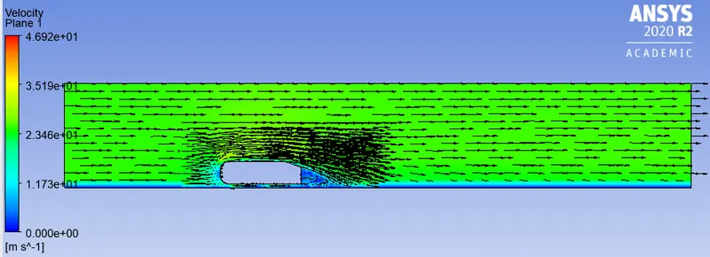
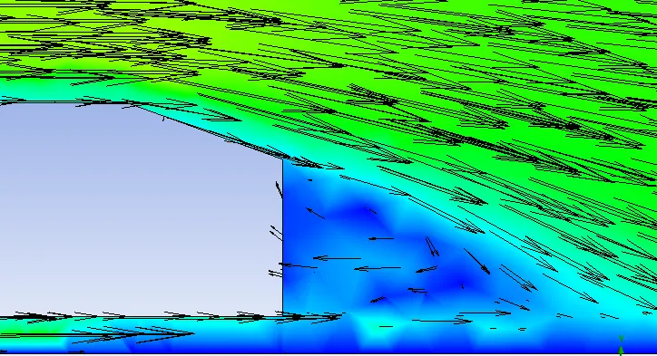
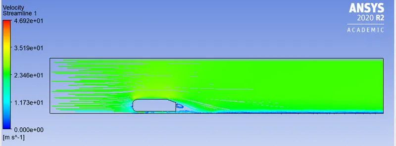
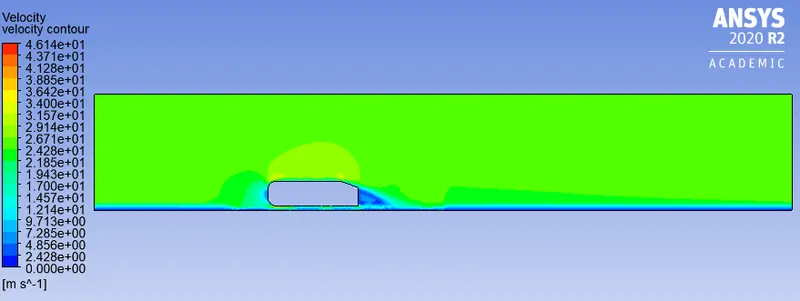
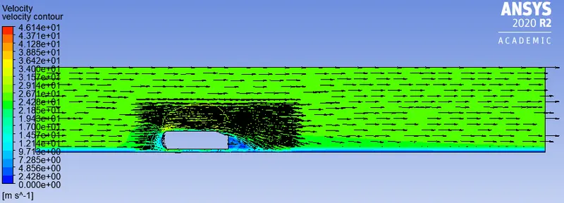
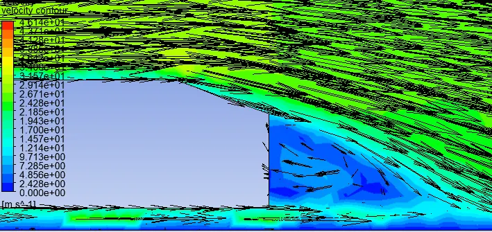
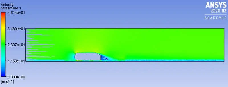
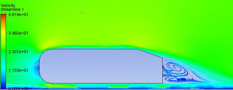
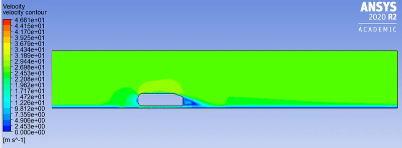
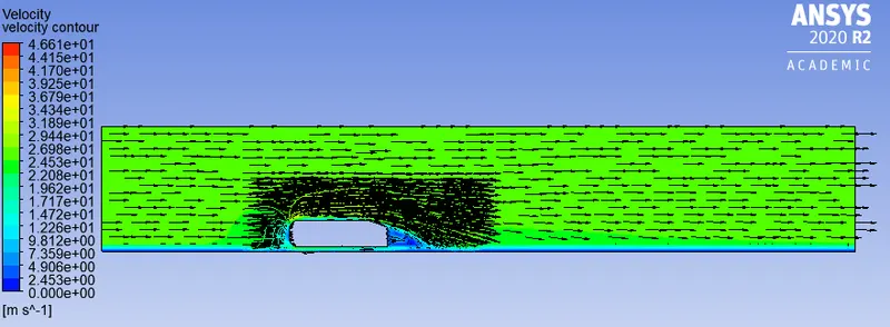
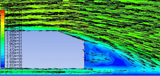
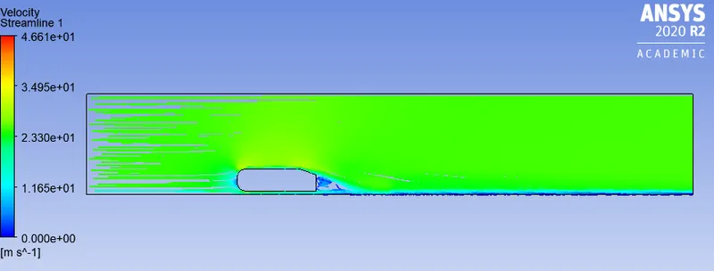
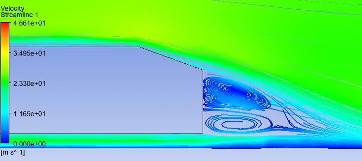
◙ From the above velocity contour plot ,vector plot and streamline plot, it is visible that the flow separates from the surface and creating a highly turbulent region behind the cylinder called the wake.
◙ Flow separation detachment of a boundary layer from a surface, which leads to the formation of wake region.
◙ From the velocity contour we can clearly observe the wake region. To understand how wake region is formed it is essential to understand what is flow separation and on what condition flow separation takes place.
◙ A flow from high pressure to low pressure (dp/dx < 0) region is always considered as favourable flow, in this case the fluid which is flowing will be decelarated by the skin friction or wall shear stress but the pressure gradient accelarates the flow.
◙ A flow where there is no pressure gradient (dp/dx = 0) there will be only decelaration because of skin friction.
◙ Thrid case is where the fluid flows from a low pressure region to high pressure region i.e, (dp/dx > 0). This is also known as adverse pressure gradient, when fluid flows under such condition both the pressure gradient as well as skin friction tries to decelarate the flow.

☻ For a flow from high pressure to low pressure i.e (dp/dx < 0) since pressure gradient accelarates the fluid flow there wont be any reverse flow, same holds good for zero pressure gradient flow.
☻ But for adverse pressure gradient flow i.e, dp/dx > 0, the pressure gradient decelarates the fluid flow so chances for flow separation and wake formation is more.
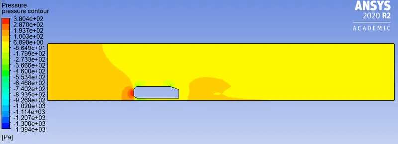
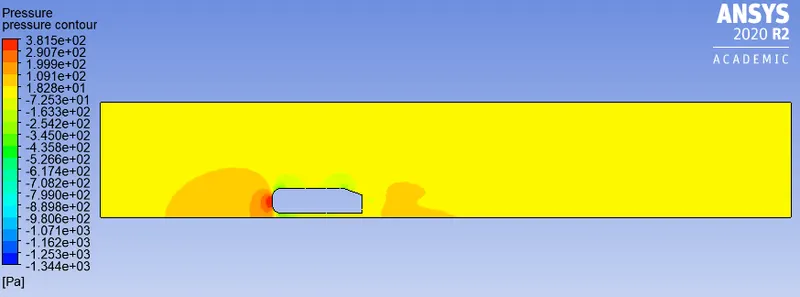
☻ Negative pressure in the wake is because we have set outlet pressure as guage pressure which is zero, since it is a adverse pressure gradient flow, pressure is increasing towards the outlet and hence negative pressure.
★ Significance of Point of Seperation :
◙ Flow separation is said to happen when the fluid flow near the wall comes to rest. These are those layers of fluid which are not on the wall but near to the wall, on the wall the layers are at rest which is called as no-slip condition.
◙ So if there is a flow separation then it's because the layers near the wall have come to rest.
◙ This can be explained by considering the velocity along y direction, velocity of the fluid at a distance dy from the wall can be given using the taylor series expansion

as we know, when flow separation takes place the layer near the wall comes to rest,i.e, 
because of no-slip condition the layer on the wall will be at rest, i.e, 
so we get,  , and hence this is the condition for flow separation.
Under such condition where , the layers near the wall resist's to flow in the direction of wall and hence flows in the opposite direction. where there is backward flow that region of flow is called wake.
◙ At this condition, velocity gradient becomes zero the wall shear stress becomes zero and hence from this point the flow separartion starts and when adverse pressure gradient is more flow reversal occurs
◙ The pressure in the wake remains close to separation-point-pressure since the eddies (formed as a consequence of the retarded layers being carried together with the upper layer through the action of shear) cannot convert rotational kinetic energy into pressure head.
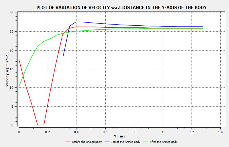
◘ Line Chart :
➦ Case - 02 : (" Grid size of 90 mm for outer enclosure & 40 mm for outer enclosure")
◙ Mesh metrics :
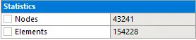
◙ Results:
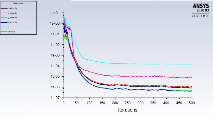
The model was initialized using Hybrid Initialization with 500 iterations to run the simulation.
◘ Residual or Convergence plot:
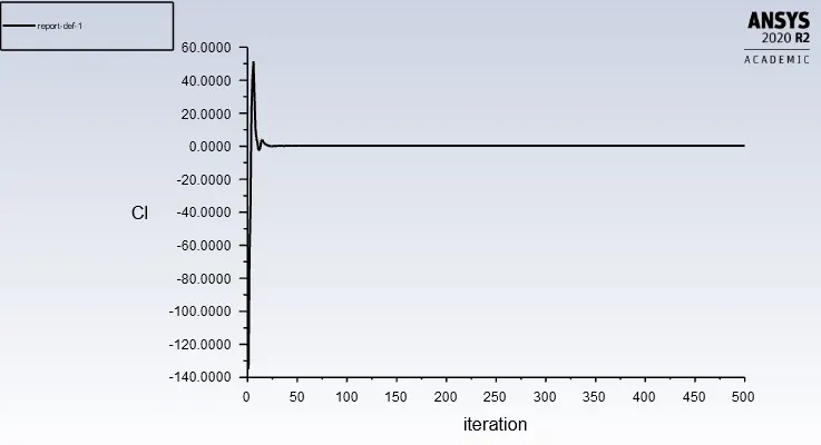
◘ Coefficient of drag(Cd) & Coefficient of lift(Cl) plots:
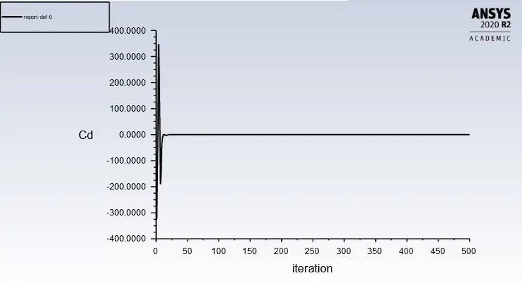
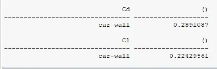
◙ The value of drag coefficient was found to be 0.289 for an inlet velocity of 25 m/s.
◙ The value of lift coefficient was found to be 0.224 for an inlet velocity of 25 m/s.
◘ Velocity Contour plot :
◘ Velocity Vector plot :
◘ Velocity Streamline plot :
◘ Pressure Contour plot :
◘ Line Chart :
➦ Case - 03 : (" Grid size of 80 mm for outer enclosure & 30 mm for outer enclosure")
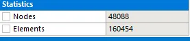
◙ Mesh metrics :
◙ Results:
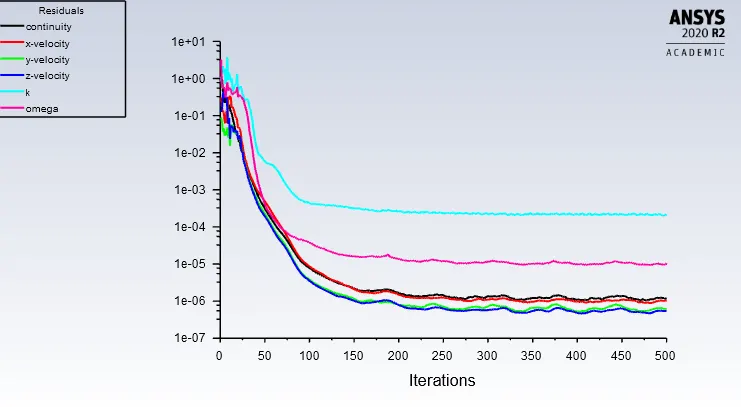
The model was initialized using Hybrid Initialization with 500 iterations to run the simulation.
◘ Residual or Convergence plot:
◘ Coefficient of drag(Cd) & Coefficient of lift(Cl) plots:
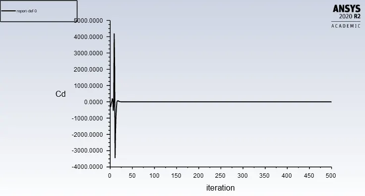
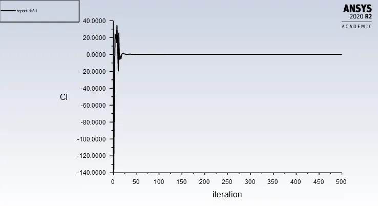
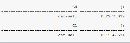
◙ The value of drag coefficient was found to be 0.278 for an inlet velocity of 25 m/s.
◙ The value of lift coefficient was found to be 0.196 for an inlet velocity of 25 m/s.
◘ Velocity Contour plot :
◘ Velocity Vector plot :
◘ Velocity Streamline plot :
◘ Pressure Contour plot :
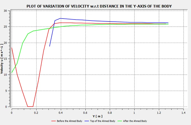
◘ Line Chart :
➦ Grid independency test :
(4) Conclusion :
★ We observed that a wake region(a large recirculation region) have established at the rear side of Ahmed body in velocity flow, Which have created a vortex flow at rear side. In that wake region, a negative pressure have been orginated. This is because of recirculation region that have been developed at the rear side of the Ahmed body.
★ Due to flow seperation behind the ahmed body we observe negative pressure because seperation of flow takes place in that area. The viscosity and the pressure gradient all together play a major role in the generation of negative pressure in the rear part or the wake region.
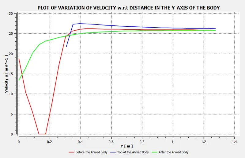
★ Apart from this wake region, We see other two small recirculation zones at curve edge of front side and the slant edge of the Ahmed body in pressure profile Known as point of separation. The point of separation is again due to the turbulence in the region. The significance for this point of separation is that it leads to deattachment of flow in the fluid which causes a sudden dropwise in stream velocity and even becomes zero at the centre of vortex in wake region. The impact of this point of separation is that it has affected flow upto 200mm of distance from rear side of body.
★ The velocity and pressure contours along with its plots in the required region has been discussed along with its significance in the report.
★ Thus the Cd and Cl values as obtained from the grid independency test shows in the above table.
★ The value of Cd does vary slightly when we go from the coarser mesh to the refined mesh case.