CFD ANALYSIS OF A MIXING TEE EFFICIENCY USING ANSYS FLUENT
Objective :
To set up the steady-state simulations to compare the mixing effectiveness of a mixing tee when hot inlet temperature is 36°C the Cold inlet is at 19°C for different cases using Ansys Fluent.
The main objective is :
(1) To Find out the average temperature at the outlet of a geometry.
(2) To compare the RANS based turbulence models (K-epsilon & K-omega).
(3) To compare cell count, No.of iterations for convergence and outlet temperature for the two cases.
(4) To perform mesh independent study for any one case.
(5) To discuss the effect of length and momentum ratios on results.
(6) To plot the Velocity and Temperature contour plots and line plots along and across the length of the pipe.
Introduction :
A tee joint is a connection of two members approximately perpendicular to one another, forming two right angles similar to the letter T. In this case there are two inlets which are oriented in x & y directions, perpendicular to each other. Mixing Tee utilizes a specifically engineered internal geometry to efficiently mix two fluid streams into one combined stream.
In this project, We're simulating the flow through a MIxing Tee in order to measure the effectiveness of mixing. The outside air comes through one of the inlets and the chilled air come through the other inlet. By adjusting the flowrate of chilled air we can get the desired temperature at the outlet. CFD approach is applied to predict the outlet temperature and velocity of the pipe at a steady state condition. In order to capture the turbulence , RANS based solver K-epsilon & K-omega turbulence models have used. By using different momentum ratios and physical parameters like cell count, No.of iterations for convergence, area weighted average, standard deviation of temperature at the outlet is predicted.
Software Used : Ansys 2020 R2
Ansys work flow for this project :
1.Geometry Setup :
◙ Two geometries have been used in this project. These computational models is uploaded to the Ansys Space Claim geometry using the step file format.
i.Short Mixing Tee Pipe : ii.Long Mixing Tee Pipe
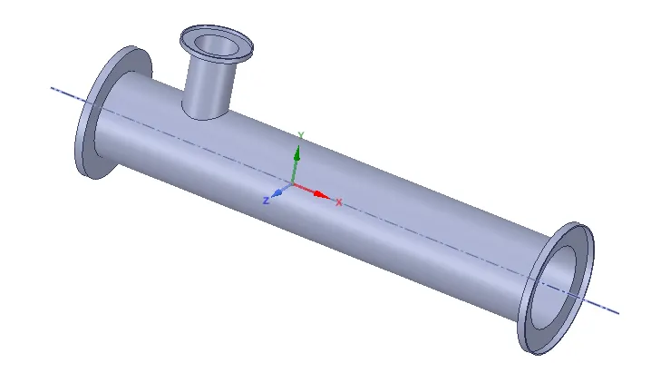
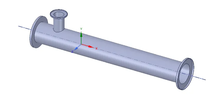
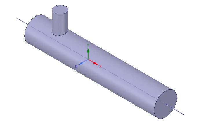
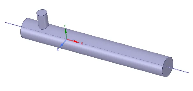
◙ In this project, our interest is to perform flow simulation so we don't need some features. We need to extract the fluid volume. Basically, 'Space Claim' is a CAD cleanup software which is very helpful for preparing a CAD model for further simulation. So by using the Fluid volume extraction utility in space claim extract the fluid domain by selecting respective edges. Then supress the solid model from the fluid model to create mesh at the interested region.
2.Mesh Generation:
◙ After loading the geometry into the workbench, Perfrom a series of operations in meshing part.
◙ Using the named selection option define the inlet_x, inlet_y, outlet, and wall.
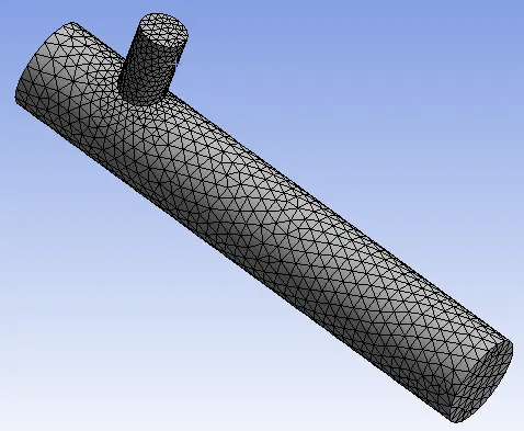
◙ Mesh size: 10 mm Mesh type : Tetrahedral mesh
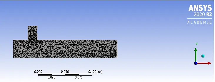
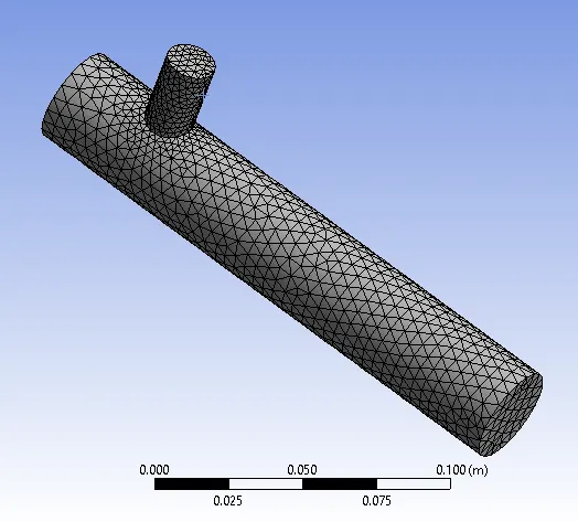
◙ After generating the mesh successfully, investigate the statistics related to elements and nodes by clicking the statistics option. Then check the mesh quality by clicking the mesh metrics option in quality section. Check whether we achieved good quality or not.
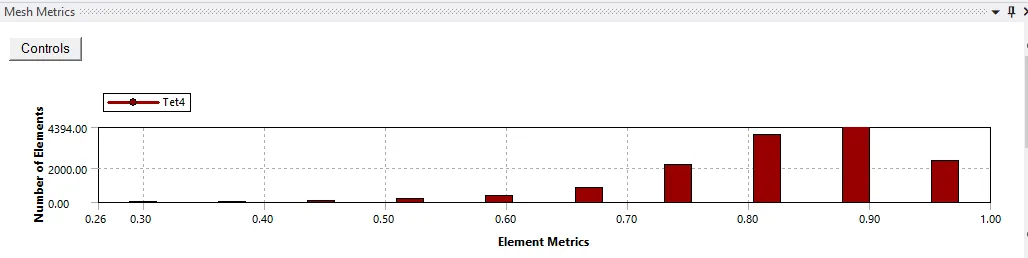
◙ Element quality is one of the important criterias in order to solve governing equations. It should not be less than 5%. In our case min mesh quality is 30%, So its quite fine to move further analysis.
3. Setup & Solution :
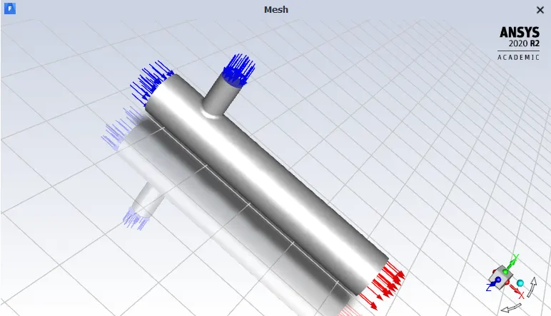
◘ CASE-01 :
➦ Short mixing Tee with a hot inlet velocity of 3m/s.
➦Momentum ratio of 2,4.
◙ Turbulence Models :
Most of the CFD problems are based on turbulence modelling. The RANS based turbulence models which were applied to the present problem:
K-epsilon model - This is one of the most common CFD models used for turbulent flow modelling. This model basically utilizes two transport variable properties K- which is
the turbulent kinetic energy and epsilon- which is the rate of dissipation of kinetic energy.
K-omega model - This is also one of the common RANS based solver used in turbulent flow problems. This model attempts to predict tubulence by solving two different
partial differential equations, which is K( Turbulent kinetic energy) and omega( Specific rate of dissipation of energy ).
◙ ( K-epsilon model predicts the turbulence parameters well far from the boundaries(wall) and K-omega model predicts the turbulence parameters well near wall)
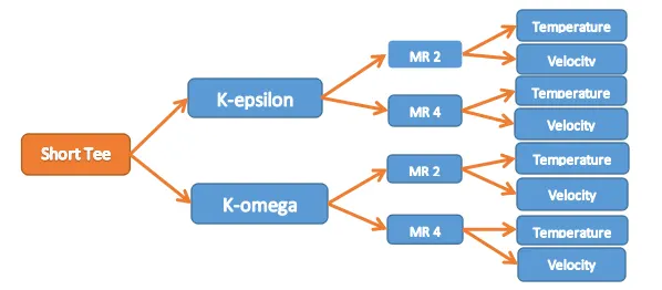
◙ Apply the both turbulence models K-epsilon realizable and K-omega SST model for the Case-01. Based on the results, use the more suitable model for Case-02.
◙ Momentum Ratio : The ratio of velocity at cold inlet to that of velocity at hot inlet.
◙ Flowchart for Turbulence model Selection :
◘ Case 1.1: Tee - short with K-epsilon realizable :
➦ Momentum ratio 2 :
◙ Solver : Pressure based
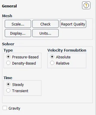
From General tab, Select the pressure-based solver along with absolute velocity formulation and with a steady state condition.
◙ Fluid : Air is the fluid in the fluid domain
◙ Energy parameter is activated since the temperature change phenomenon needs to be studied in this case.
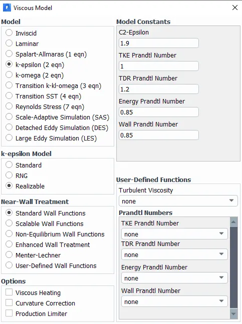
◙ Turbulence Model : Select the viscous model which is K-epsilon realizable.
◙ Boundary conditions:
• Hot inlet Temperature - 36°C
• Cold inlet Temperature - 19°C
• Hot inlet air velocity - 3m/s
• Cold inlet air velocity - 6m/s (i,e.. Momentum Ratio = 2)
• Outlet : Pressure outlet type, 0 gauge pressure
• Walls: Wall type, No slip condition
◙ Initialize the solver with hybrid schemes. And setup No.of iterations and then click on calculate option.
◘ Results :
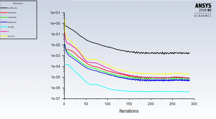
➦ Convegence plot :
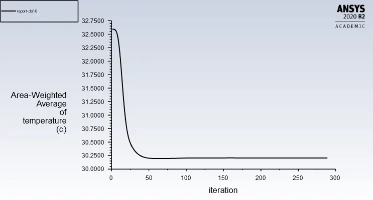
➦ Area weighted average of temperature :
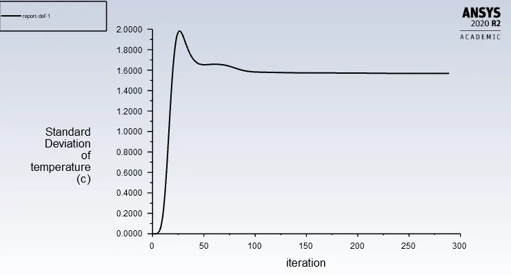
➦ Standard deviation of temperature :
◘ Post processing results :
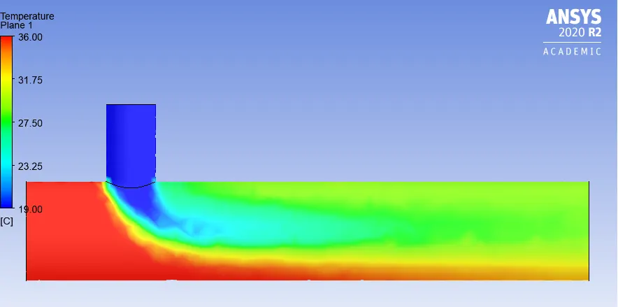
➦ Temperature contour along the pipe :
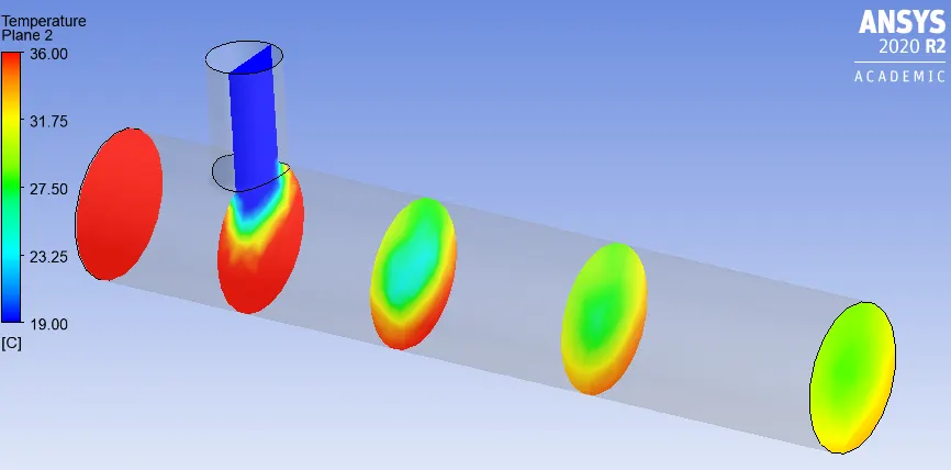
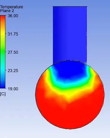
➦ Temperature contour across the pipe :
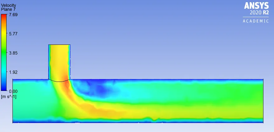
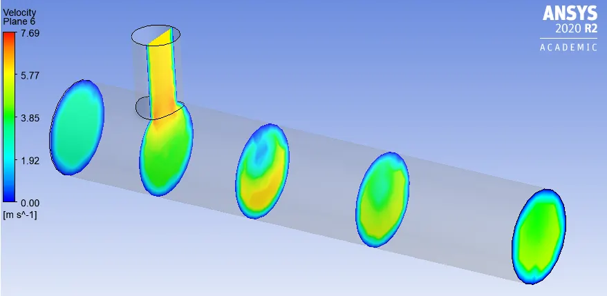
➦ Velocity contour along the pipe :
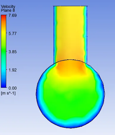
➦ Velocity contour across the pipe :
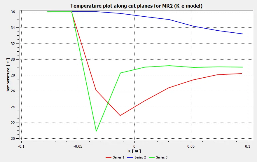
➦ Temperature line plot along the pipe :
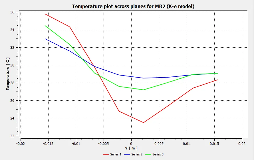
➦ Temperature line plot across the pipe :
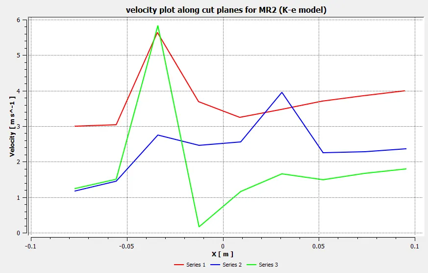
➦ Velocity line plot along the pipe :
➦ Velocity line plot across the pipe :
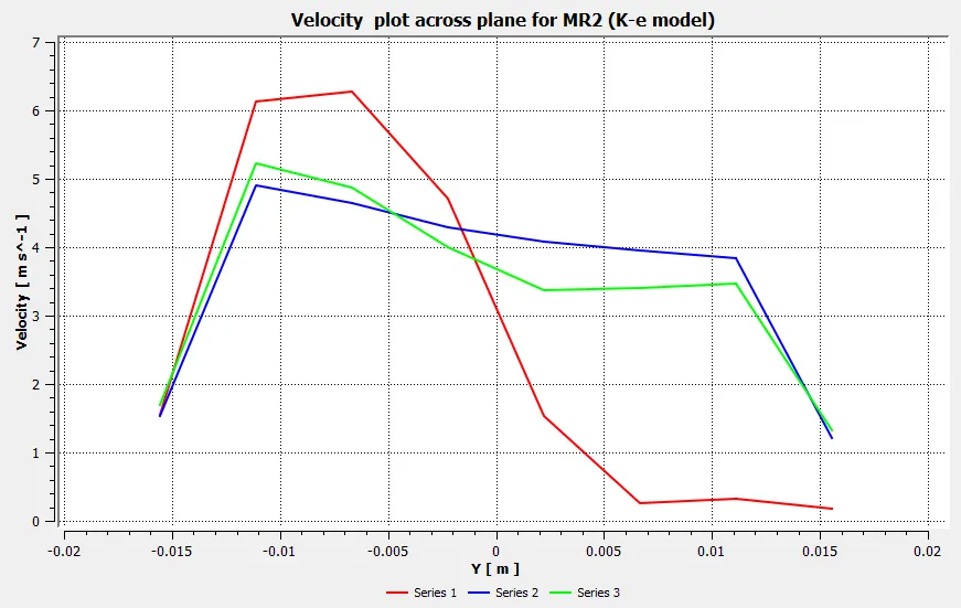
◙ The post processing results shows the variation of temperature and velocity along and across the length of the pipe.
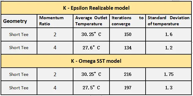
◙ The average outlet temperature becomes 30.25°C, Solution get converged at 150th iteration and standard deviation of temperature is 1.6
➦ Momentum ratio 4 :
• Change the Cold inlet air velocity to - 12m/s (i,e.. Momentum Ratio = 4). Keep the others as same as before.
◙ Initialize the solver with hybrid schemes. And setup No.of iterations and then click on calculate option.
◘ Results :
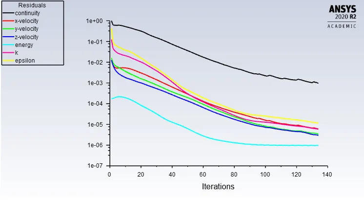
➦ Convegence plot :

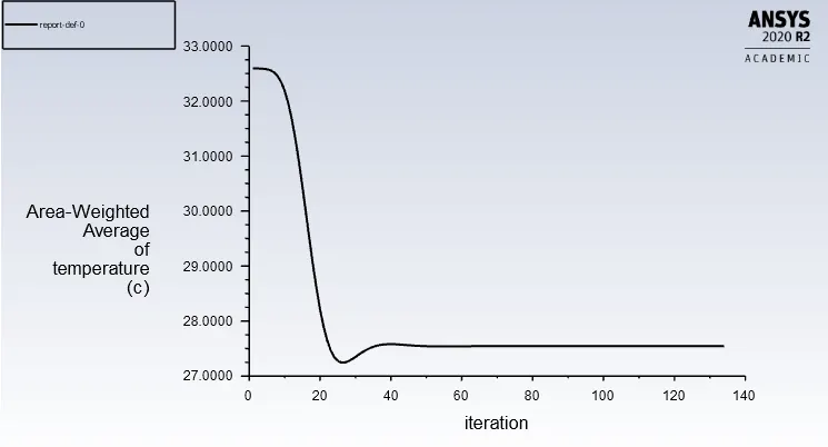
➦ Area weighted average of temperature :
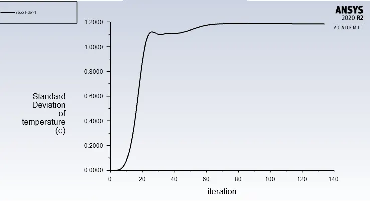
➦ Standard deviation of temperature :
◘ Post processing results :
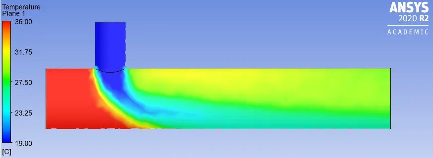
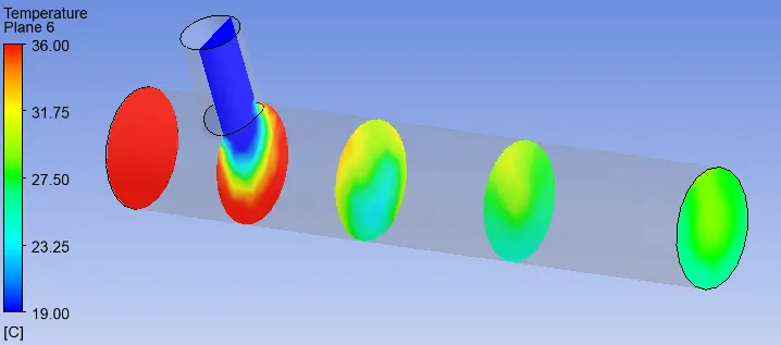
➦ Temperature contour along the pipe :
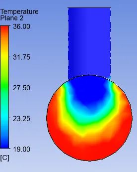
➦ Temperature contour across the pipe :
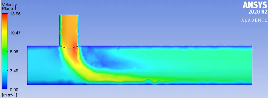
➦ Velocity contour along the pipe :
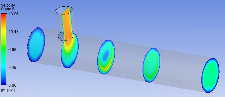
➦ Velocity contour across the pipe :
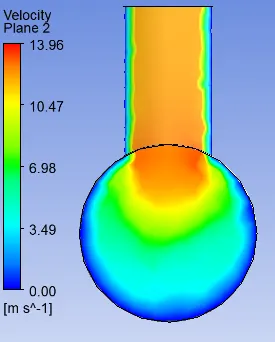
➦ Temperature line plot along the pipe :
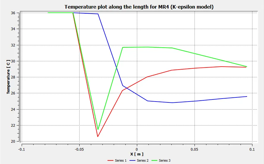
➦ Temperature line plot across the pipe :
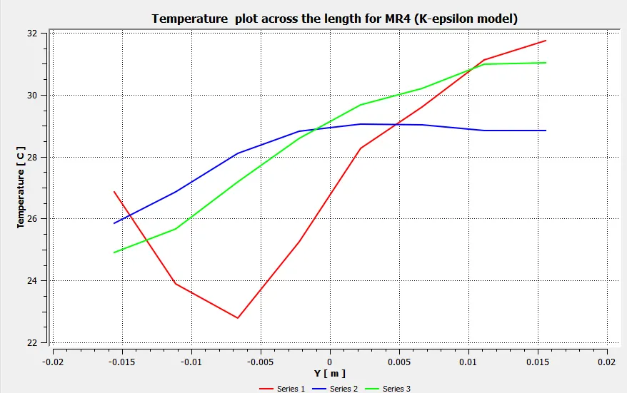
➦ Velocity line plot along the pipe :
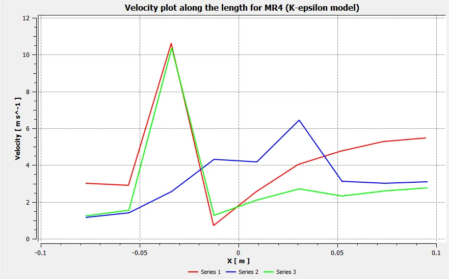
➦ Velocity line plot across the pipe :
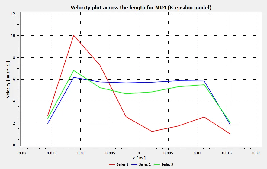
◙ The post processing results shows the variation of temperature and velocity along and across the length of the pipe.
◙ The average outlet temperature becomes 27.5°C, Solution get converged at 134th iteration and standard deviation of temperature is 1.2
◘ Case 1.2: Tee - short with K - omega SST :
➦ Momentum ratio 2 :
◙ Select the K - omega SST turbulence model
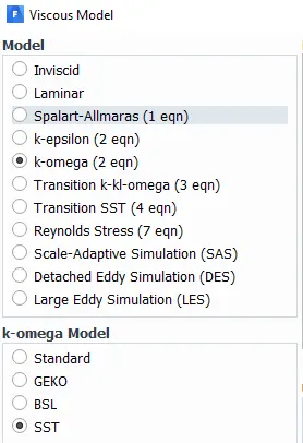
◙ Set the boundary conditions and initialize the solver with hybrid schemes. And setup No.of iterations and then click on calculate option.
◘ Results :
➦ Convegence plot :

➦ Area weighted average of temperature :
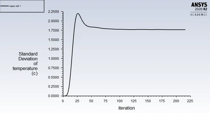
➦ Standard deviation of temperature :
◘ Post processing results :
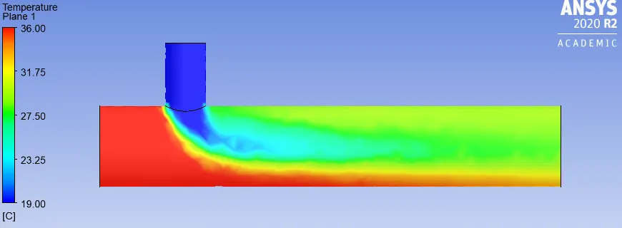
➦ Temperature contour along the pipe :
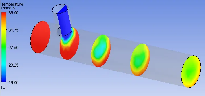
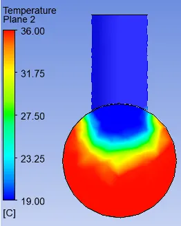
➦ Temperature contour across the pipe :
➦ Velocity contour along the pipe :
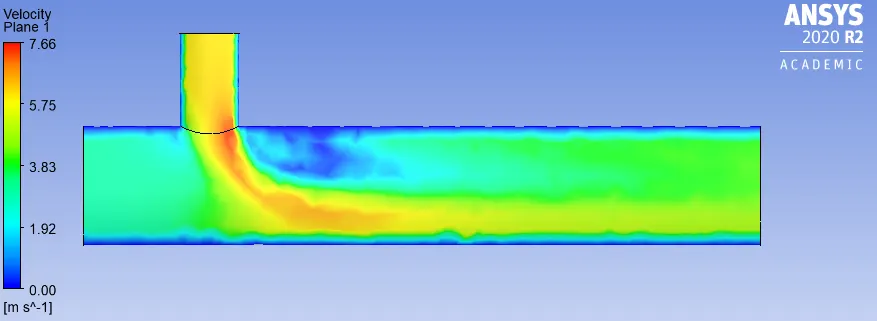
➦ Velocity contour across the pipe :
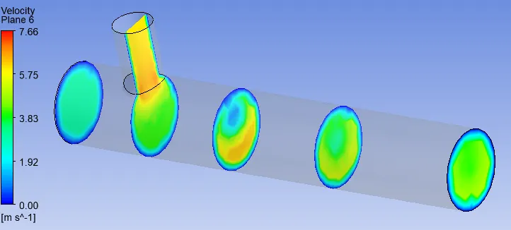
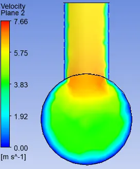
➦ Temperature line plot along the pipe :
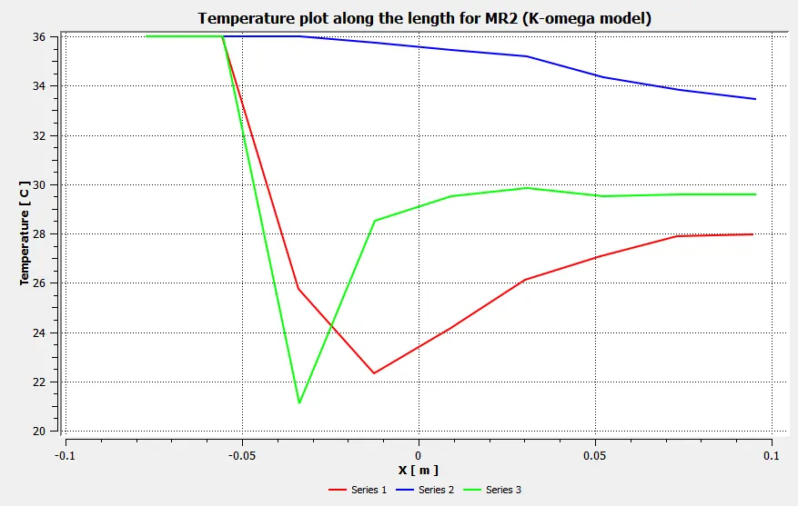
➦ Temperature line plot across the pipe :
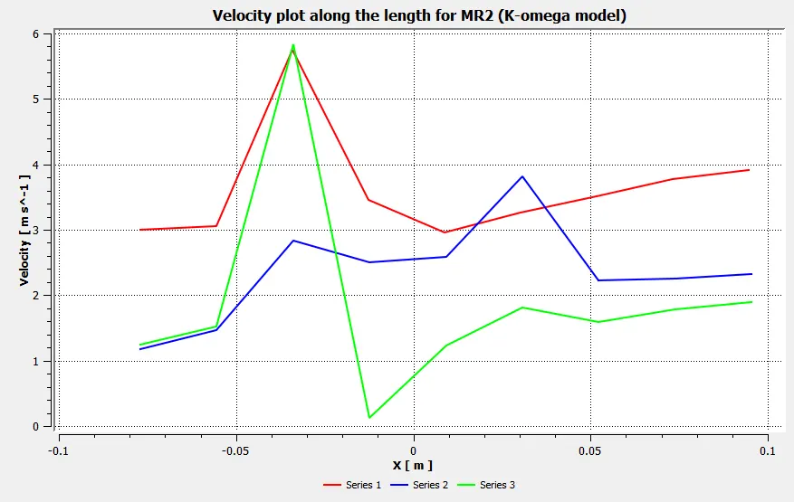
➦ Velocity line plot along the pipe :
➦ Velocity line plot across the pipe :
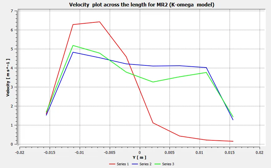
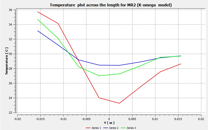
◙ The post processing results shows the variation of temperature and velocity along and across the length of the pipe.
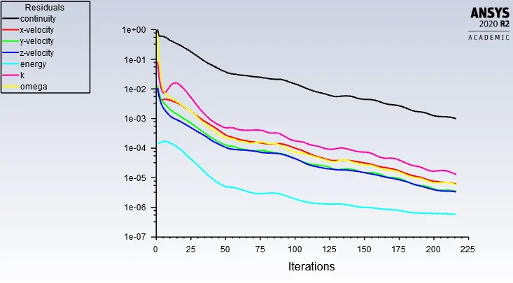
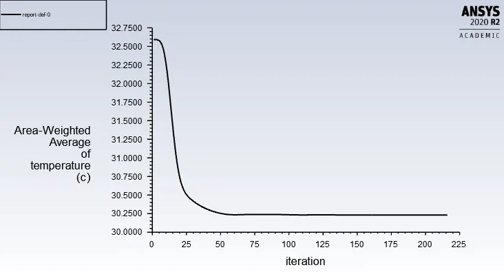
◙ The average outlet temperature becomes 30.25°C, Solution get converged at 216th iteration and standard deviation of temperature is 1.75.
➦ Momentum ratio 4 :
◙ Change the Cold inlet air velocity to - 12m/s (i,e.. Momentum Ratio = 4). Keep the others as same as before.
◙ Initialize the solver with hybrid schemes. And setup No.of iterations and then click on calculate option.
◘ Results :
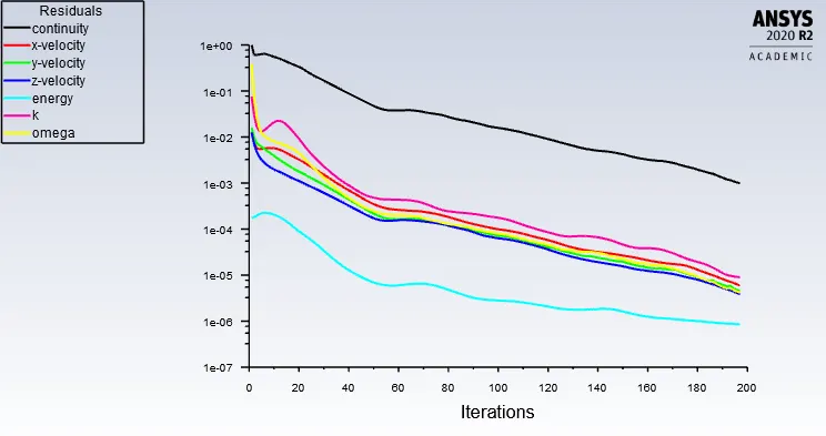
➦ Convegence plot :

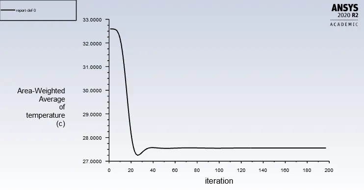
➦ Area weighted average of temperature :
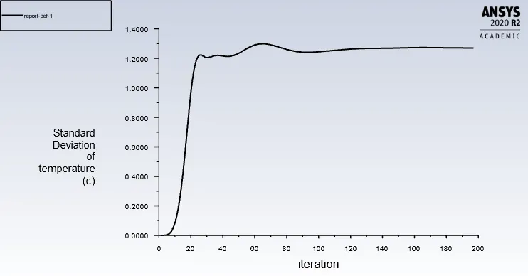
➦ Standard deviation of temperature :
◘ Post processing results :
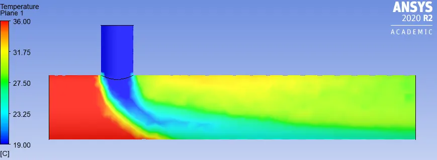
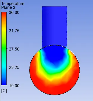
➦ Temperature contour along the pipe :
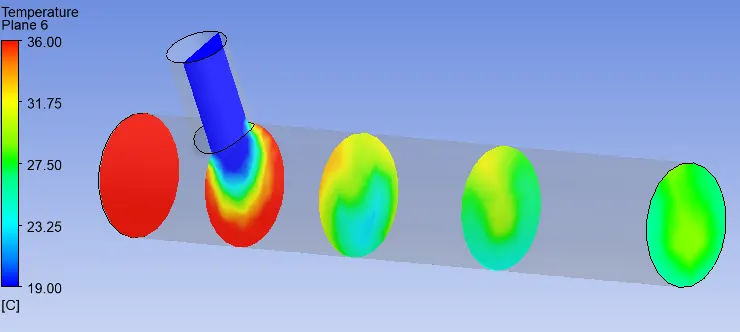
➦ Temperature contour across the pipe :
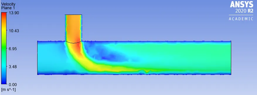
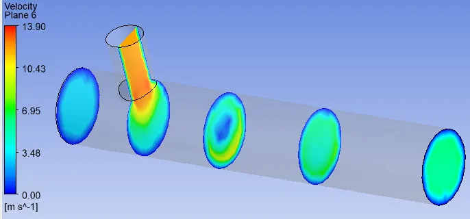
➦ Velocity contour along the pipe :
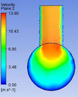
➦ Velocity contour across the pipe :
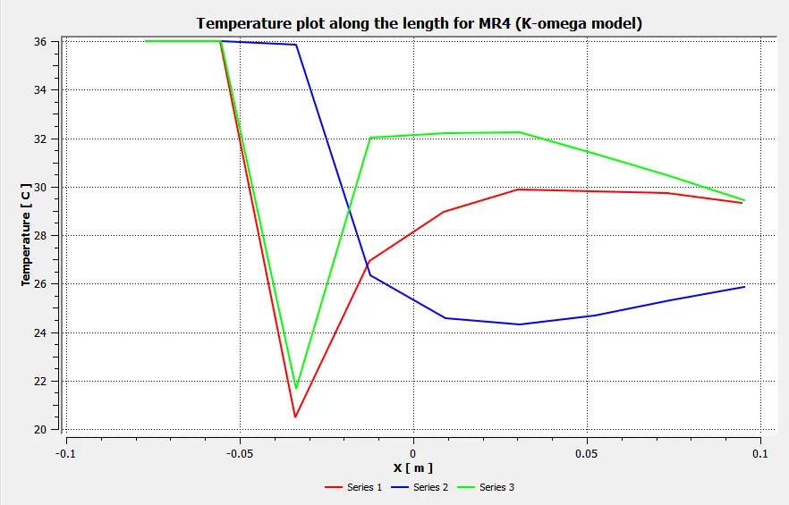
➦ Temperature line plot along the pipe :
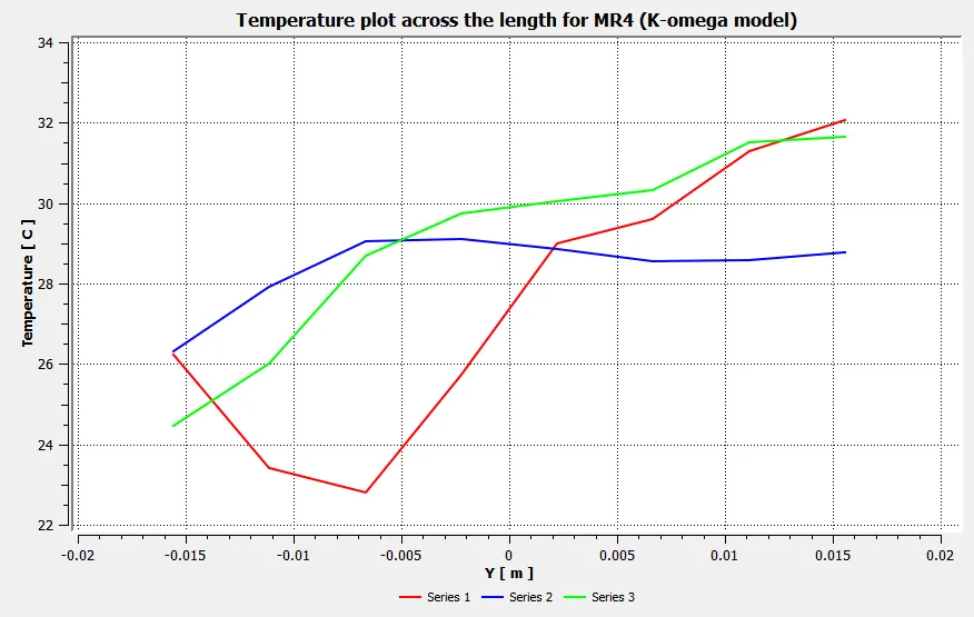
➦ Temperature line plot across the pipe :
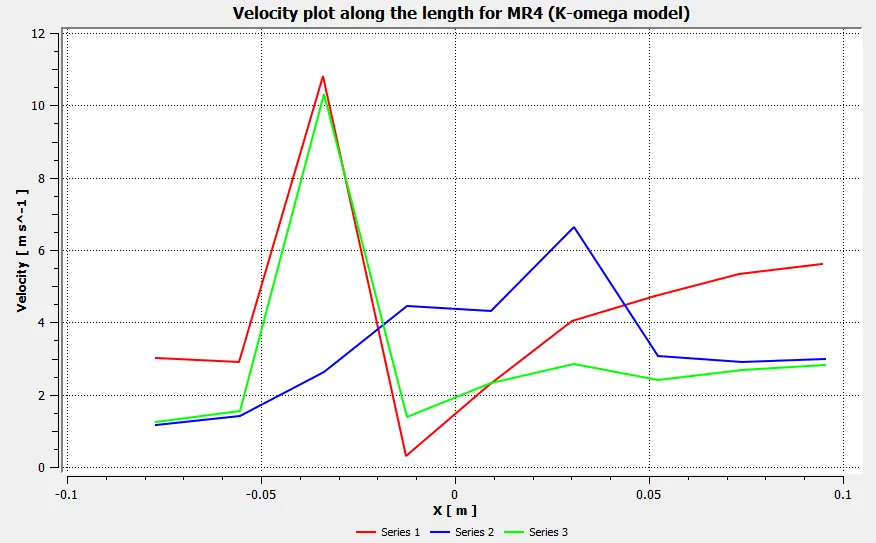
➦ Velocity line plot along the pipe :
➦ Velocity line plot across the pipe :
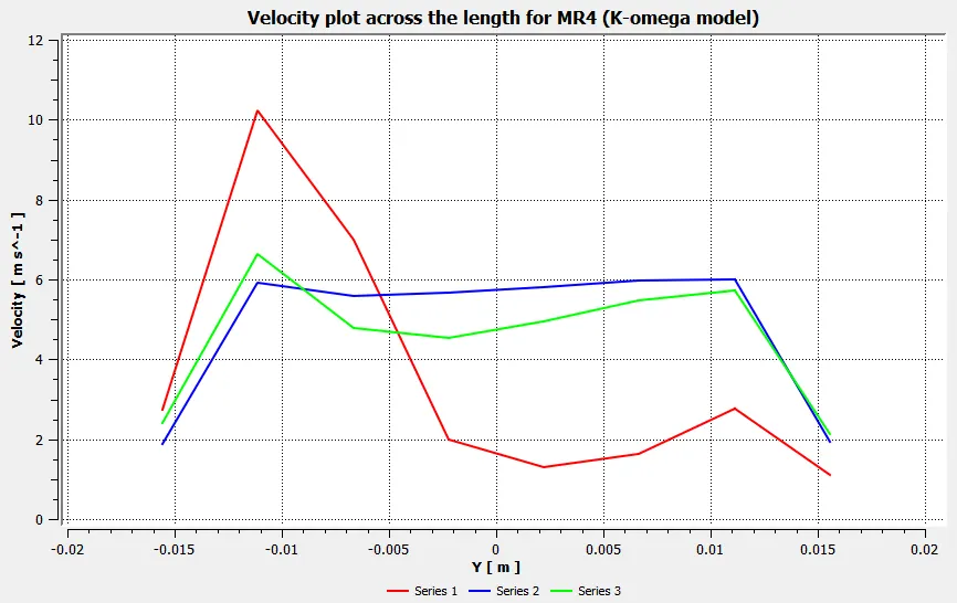
◙ The post processing results shows the variation of temperature and velocity along and across the length of the pipe.
◙ The average outlet temperature becomes 27.5°C, Solution get converged at 197th iteration and standard deviation of temperature is 1.3.
◘ Comparison between the both turbulent models for short Tee geometry with analytical solution :
◘ Analytical Solution :
➦Momentum Ratio 2 :
⟾ Mass of hot fluid (mh) = ρ* A* Vh= 997*0.0009*3 = 2.69 kg/s
⟾ Mass of cold fluid (mc) = ρ* A* Vc= 997*0.0009*6 = 1.35 kg/s
⟾ Temperature of mixture (Tmixture) = (mh * Th + mc * Tc) / (mc + mh) = 30.319°C
➦Momentum Ratio 4 :
⟾ Mass of hot fluid (mh) = ρ* A* Vh= 997*0.0009*3 = 2.69 kg/s
⟾ Mass of cold fluid (mc) = ρ* A* Vc= 997*0.0009*12 = 2.3928 kg/s
⟾ Temperature of mixture (Tmixture) = (mh * Th + mc * Tc) / (mc + mh) = 27.99°C
◘Conclusions :
♢ Avg. outlet temperature: On comparing the two tubulent models from the analytical solution, we got nearly same results.
♢ Iterations to converge: No.of iterations taken by K-Omega SST to achieve convergence is higher than that taken by the K-epsilon realizable model.
♢ Standard deviation of temperature: K-Omega SST model produced higher standard deviation that means less accuracy in predicting results for this model.
♢ K-epsilon provides standard results for overall region. If we are interested to capture the phenomenon in such regions nearer to wall, in such a case we should use K-omega with very fine meshing near to wall.
◘ So based on above conclusions, it is recommended to use k-epsilon realizable turbulence model since it is predicting the results very accurately within less iterations.
☻ Case 2 : Long mixing Tee with a hot inlet velocity of 3m/s,
Momentum of ratio of 2,4.
◘ Case 2.1: Tee - Long with K-epsilon realizable :
⟾ Turbulence Model : Select the K-epsilon realizable Viscous model.
➦ Momentum ratio 2 :
◙ Set the conditions as above and initialize the solver with hybrid schemes. And setup No.of iterations and then click on calculate option.
◘ Results :
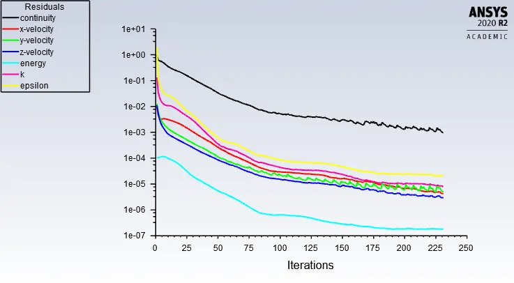
➦ Convegence plot :

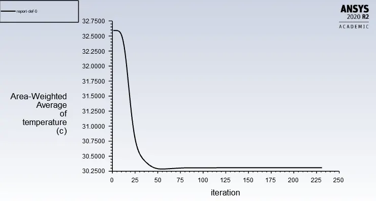
➦ Area weighted average of temperature :
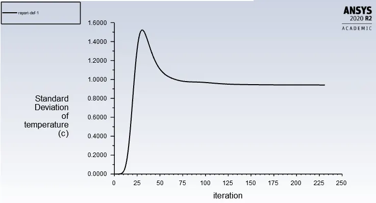
➦ Standard deviation of temperature :
◘ Post processing results :
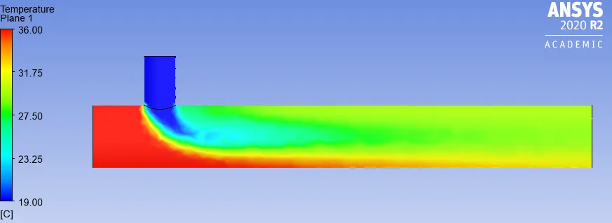
➦ Temperature contour along the pipe :
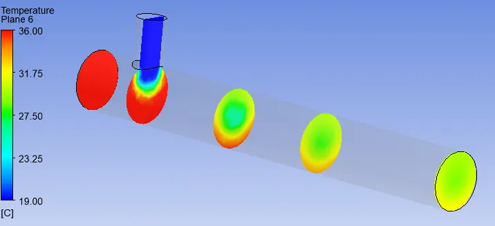
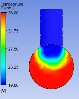
➦ Temperature contour across the pipe :
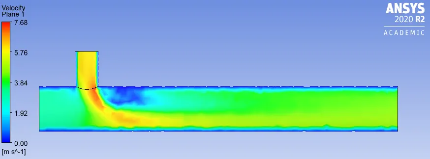
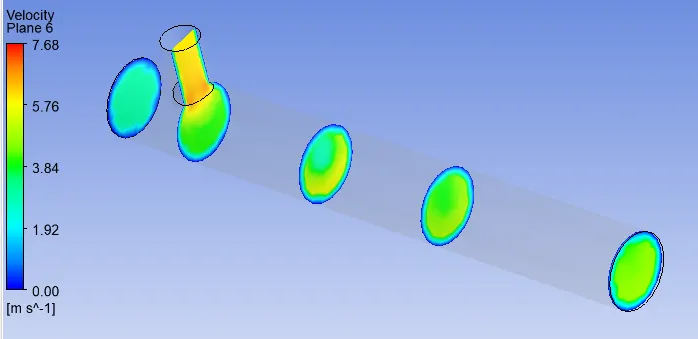
➦ Velocity contour along the pipe :
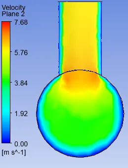
➦ Velocity contour across the pipe :
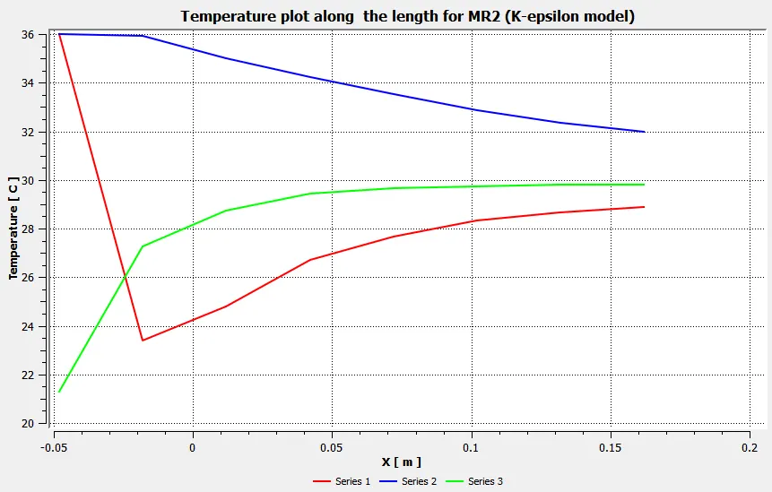
➦ Temperature line plot along the pipe :
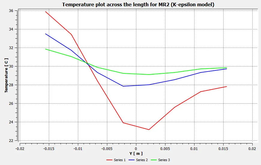
➦ Temperature line plot across the pipe :
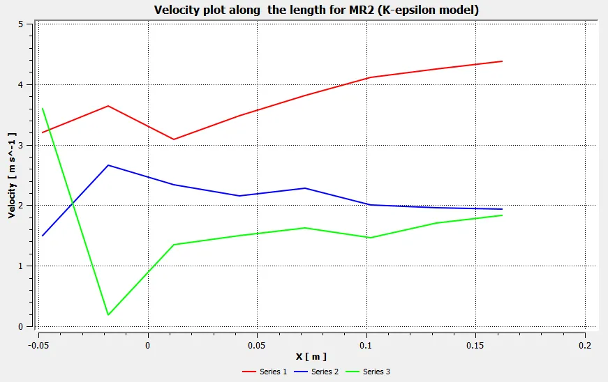
➦ Velocity line plot along the pipe :
➦ Velocity line plot across the pipe :
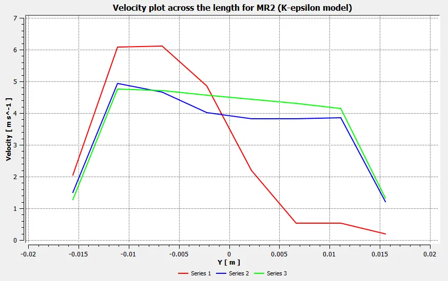
◙ The post processing results shows the variation of temperature and velocity along and across the length of the pipe.
◙ The average outlet temperature becomes 30.30°C, Solution get converged at 231th iteration and standard deviation of temperature is 0.9
➦ Momentum ratio 4 :
◙ Change the Cold inlet air velocity to - 12m/s (i,e.. Momentum Ratio = 4). Keep the others as same as before.
◙ Initialize the solver with hybrid schemes. And setup No.of iterations and then click on calculate option.
◘ Results :
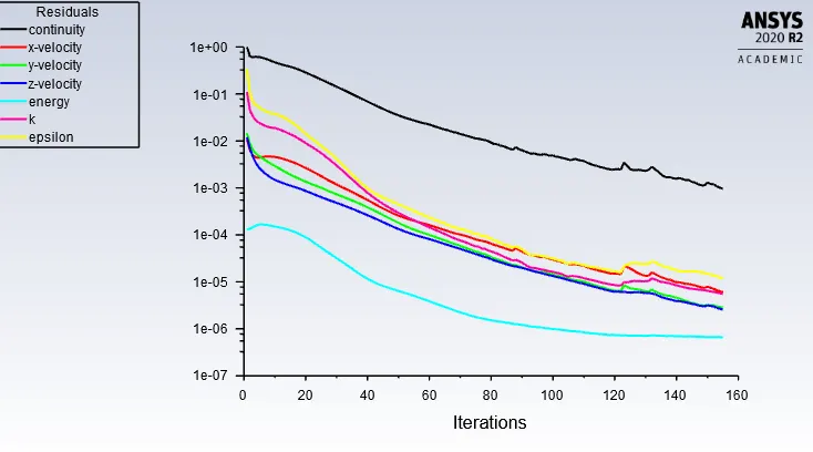
➦ Convegence plot :

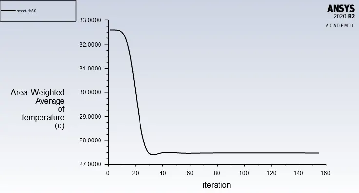
➦ Area weighted average of temperature :
➦ Standard deviation of temperature :
◘ Post processing results :
➦ Temperature contour along the pipe :
➦ Temperature contour across the pipe :
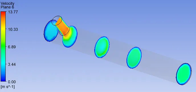
➦ Velocity contour along the pipe :
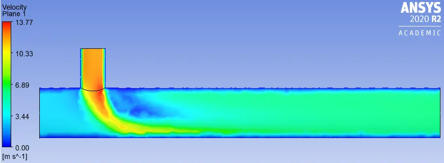
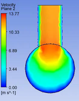
➦ Velocity contour across the pipe :
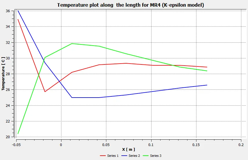
➦ Temperature line plot along the pipe :
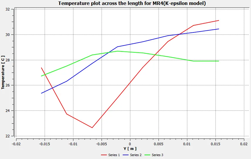
➦ Temperature line plot across the pipe :
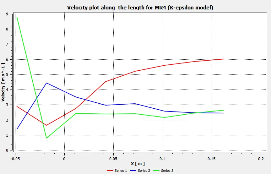
➦ Velocity line plot along the pipe :
➦ Velocity line plot across the pipe :
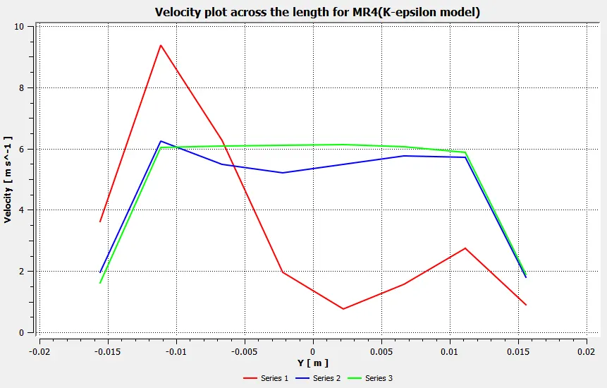
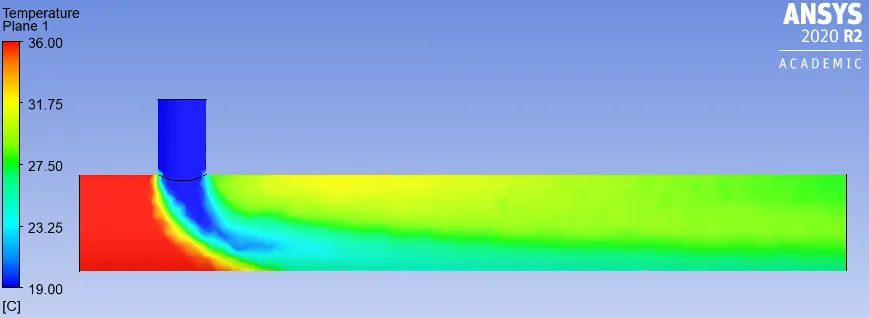
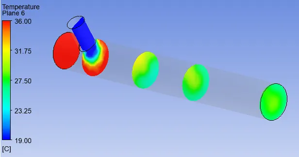
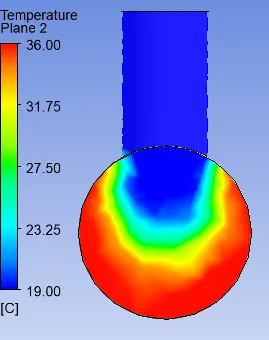
◙ The post processing results shows the variation of temperature and velocity along and across the length of the pipe.
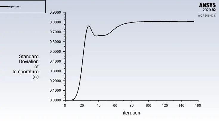
◙ The average outlet temperature becomes 27.5°C, Solution get converged at 155th iteration and standard deviation of temperature is 0.8
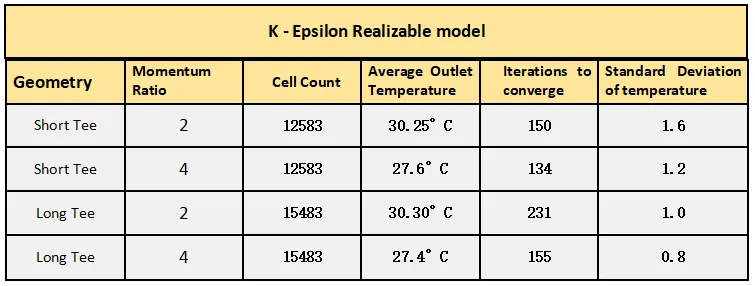
◘ Comparison between the both Geometries with analytical solution :
◘ Discussions :
♢ Avg. outlet temperature: Since we are interested on the fluid volume, the temperature at the outlet we got in case-01 and case-02 is near about the same irrespective of the length of mixing tee.
♢ Momentum Ratio :
➣ Higher the momentum ratio, cold fluid entrance velocity will be higher therefore amount of cold fluid entering the pipe also be higher, and due to higher relative velocity between the fluds it experiences higher turbulence and thereby outlet fluid temperature drops.
➣ For momentum ratio=2, the average fluid outlet temperature is around 30.3°C whereas for momentum ratio=4 it is confined to 27.5°C, so there is a drop of temperature by almost 3°C at at outlet with the use of high momentum ratio.
➣ So in order to attain better turbulent mixing, the velocity of the chilled air is very important. By increasing the velocity of chilled air the outlet temperature get reduced.
♢Iterations to converge : Longer configuration take more iterations to converge and to predict the desired results than the shorter configuration.
◘ Conclusions :
♢ Higher the momentum ratio, higher the mixing efficiency of Tee-joint.
♢ Increase in length of the pipe doesn't serve the mixing purpose efficeintly, so it's Efficient to use short pipe.
◘ Grid Independency Test :
➦Geometry Selected: Short- Tee model.
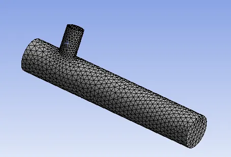
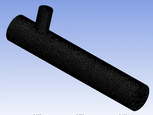
➦ Mesh Generation:
5mm 3mm 1mm
➦ Results @ Mesh 5mm :
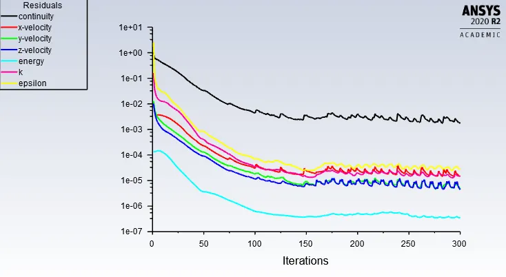
➦ Convegence plot :
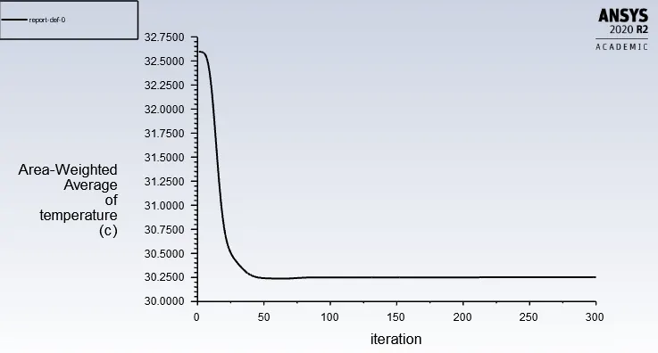
➦ Area weighted average of temperature :
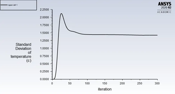
➦ Standard deviation of temperature :
➦ Results @ Mesh 3mm :
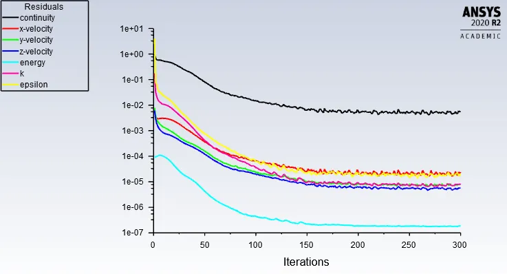
➦ Convegence plot :
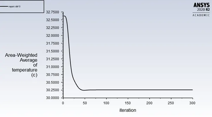
➦ Area weighted average of temperature :
➦ Standard deviation of temperature :
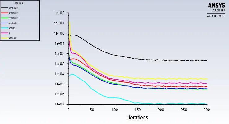
➦ Results @ Mesh 1mm :
➦ Convegence plot :
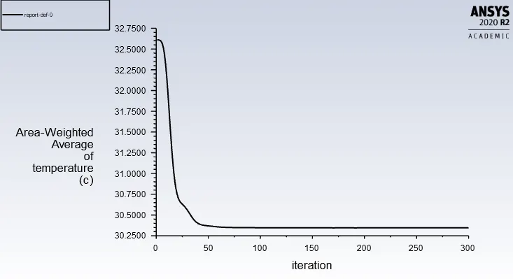
➦ Area weighted average of temperature :
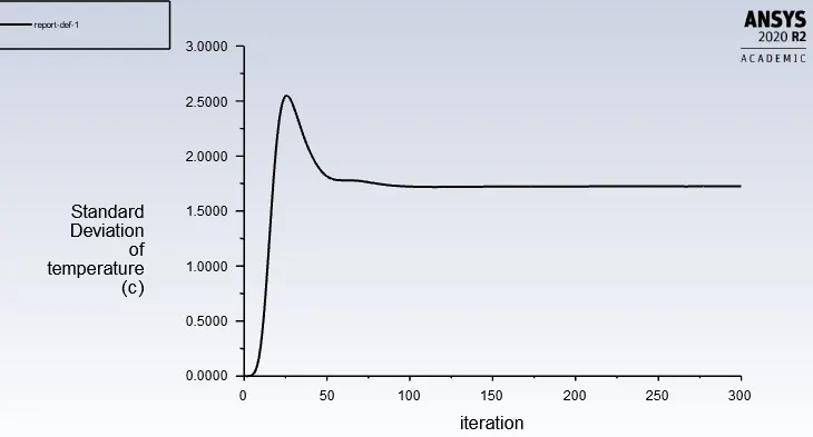
➦ Standard deviation of temperature :
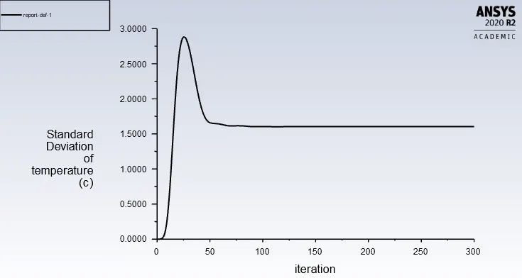
◘ Comparison between different Mesh sizes of short Tee @ MR2 :
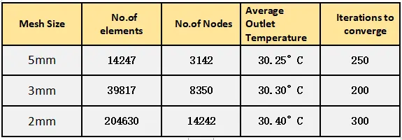
◙ Mesh Refinement :
➣ We're refining the mesh means we're adding more no.of cells. Solver going to take more iterations to converge to a particular value.
➣ Finer mesh means, more cells to be processed. More governing fluid dynamic equations are being solved on each & every cells. For this reason simulation time is increasing. Whereas mesh is coarse means, we're having few no.of cells then linear solver can converge pretty fast.
◘ Conclusion :
◙ From the grid independency test, it is seen that mesh size of 3mm gives the best predicted results as compared to other mesh sizes.
◙ It is seen that on decreasing the mesh size the average outlet temperature also starts approaching towards the analytical results. Taking too finer mesh shows deviation from the analytical solution.
◙ The mesh grid independency test shows the effect of meshing parameter on the average outlet temperature distribution.