Solving differential equation of pendulum with damping

Aim : Solving ordinary Differential equation using ode45 inbuilt function.

Objective : Algorithm to solve ordinary differential equation using ode45.

Basic knowledge of Damping.

Theory :

Genrally we neglect the losses due to drag while solving the problems.But practically

we cannot ignore them .

Let's consider simple pendulum..,

If losses are neglected then the amplitude remains constant , even with no apply

of force periodically , called natural vibrations or oscillations.

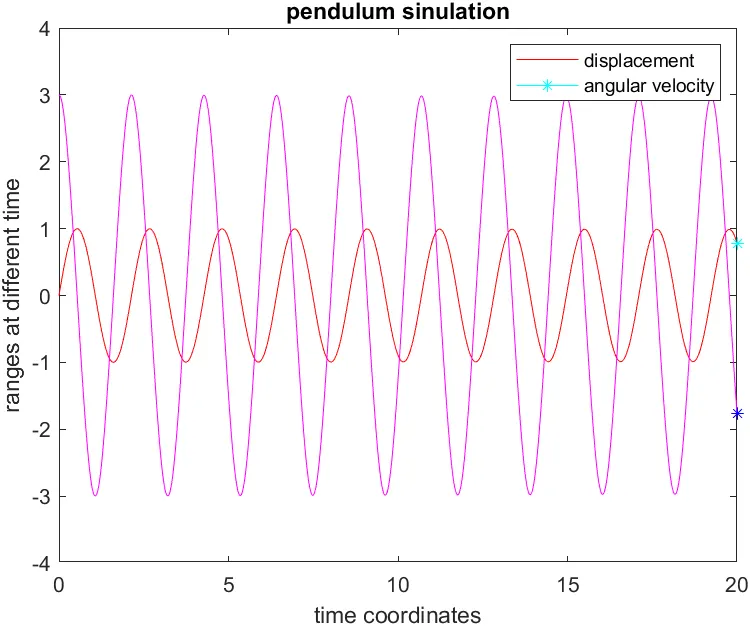
You can observe the no variation of amplitude over of cycles - if damping neglected.

In practical this is not the case , decrease in amplitude obsorved , that phenomenon

called damping.

Energy dissipates due to drag or frictional forces.

Important term in damping to differ types of damping - Damping ratio

Damping Ratio(`xi`) = `frac{Damping Coefficient}{Critical Damping coefficient (C_c)}`

Critical Damping coefficient(`C_c`) = `2sqrt(m*k)`.

Different types of Damping :

• Underdamped - `xi``lt 1`.
• Overdamped - `xi gt 1`.
• Criticaldamped - `xi = 1`.
• Undamped - `xi = 0`.

Observe the plots of types of damping

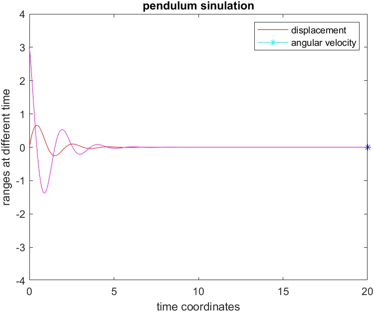
fig : Overdamping

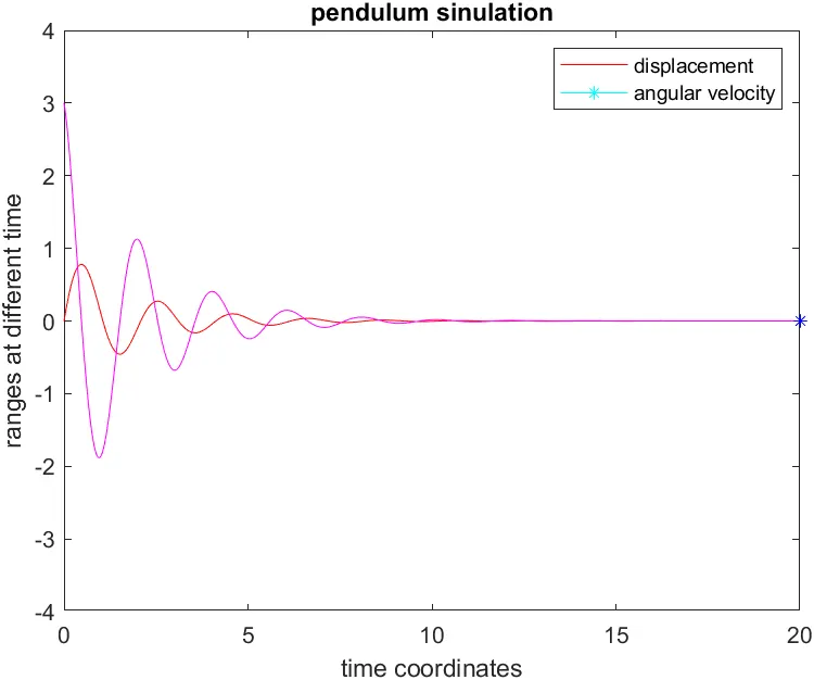
fig :Criticaldamping

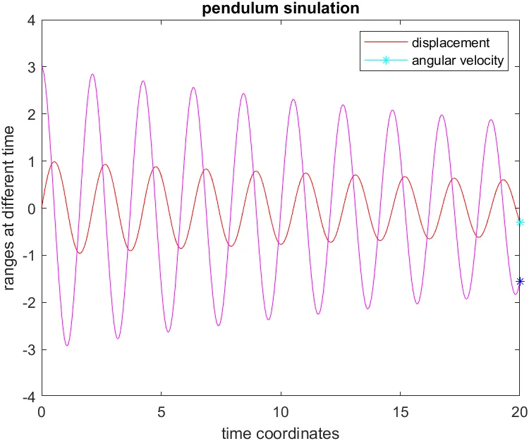
fig : underdamped

ode45 inbuilt function :

Syntax : ode45(fname , tspan , IVC , options).

fname - ode function solves the differential equation algorithm.

tspan - Interval range to integrate.

actually , t_co dimentions same as tspan , but if required for accuracy matlab can manipulate for required dimentions, change step-size.

IVC - Space coordinates , initial conditions.

In matlab , genrally ode45 use the runge-kutta (`4^(th)` order) - Numerical analysis.

Method as results are more accurate than other methods. (Rate of convergence - 2).

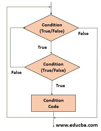
Workflow of for loop:

Description of simple pendulum under viscous damping:

Governing equation :

`frac{d^2theta}{dt^2}`+ `frac{b}{m} (frac{d theta}{dt}) + frac{g}{l}sintheta = 0`

b - Damping co-efficient.

`theta - ` angular displacement of the pendulum bob`

g - acceleration due to gravity.

l - lenght of the pendulum wire.

here , considered the viscous damping (drag due to the fluids like air,water...).

viscous damping - force is directly proportional to velocity.

`F_d = b*dotx`

b - damping coefficient.

If we neglected the term 'b' = 0 , the governing equation becomes

`frac{d^2theta}{dt} + frac{g}{l}sintheta = 0`.

This discribes the natura free vibrations without daping.

Simple pendulum figure output:

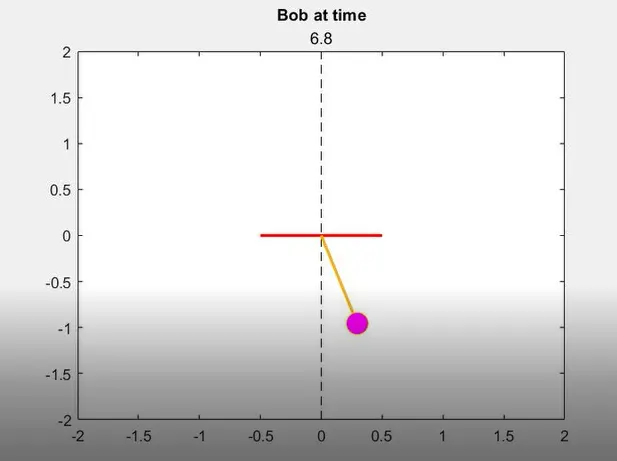
This figure shows the output plot animation of simple pendulum

Code :

%% clearing commands
close all ; clear all ; clc ;
%% Defining the input variables known
l = 1;
% time range
t_span = [0:(20/200):20];
% Space co-ordinates initial conditions
s_co = [0 ; 3];
% ode45
[t,s] = ode45(@pendulum_function , t_span , s_co);
%% plotting
% Displacement and velocity with time along x-axis
for i =1:length(s(:,1))
plot(t(1:i),s(1:i,1),'color','b')
hold on
plot(t(i),s(i,1),'marker','*','MarkerFaceColor','r')
plot(t(1:i),s(1:i,2),'color','m')
plot(t(i),s(i,2),'marker','*','MarkerFaceColor','y')
xlabel('time co-ordinates')
ylabel('quantity')
legend('displacement','velocity')
axis([0 25 -5 5])
drawnow
hold off
end
%% Animation
figure(2)
clc
for i=1:length(s(:,1))
plot([-0.5 0.5],[0 0],'color','r','LineWidth',2)
axis([-2 2 -2 2])
hold on
plot([0 0],[-4 4],'color','k','LineStyle','--')
x1(i) = l*sin(s(i,1));
y1(i) = l*cos(s(i,1));
plot([0,0+x1(i)],[0,0-y1(i)],'LineWidth',2)
plot(x1(i),-y1(i),'marker','o','MarkerFaceColor','m','MarkerSize',15,'MarkerEdgeColor','y')
title('Bob at time',num2str(t(i,1)))
drawnow
hold off
fr(i) = getframe(gcf);
end
%VideoWriter used to create the videofile.
%Use a VideoWriter object to create a video file from an array or MATLAB movie.
%The object contains information about the video and the properties that control the output video.
video_file = VideoWriter('fra');
%open the videofile.
open(video_file)
%writeVideo to create the video using the data stored in 'fr'.
writeVideo(video_file,fr)
%close the videofile.
close(video_file)

Explanation of code step-wise :

1.At first , used genral commands ,

close all - to clear all existing figures and plots.

clear all - to remove all data in workspace.

clc - to clear the command prompt.

2.Defined length of pendulum wire , assigned to variable 'l'.

3.tspan - time interval range over integration ocuurs.

4.S0 - Defining Space coordinates.

5.Use ode45 inbulit function to solve the ordinary differential equation , syntax explained above.

6.Results stored in t_co - time coordinates , re - dispacement and velocity of oscillations values along columns.

7.used first for loop to plot the displacement and velocity variations over cycles with time(x-axis).

8.used the second for loop to show the animation of simaple pendulum with taken underdamped condition.

9.hold on - add the present axes properties to the current figure.

10.drawnow - hold the execution of code temporarly and plot the present figure , as matlab gives prference to the execution of code.

11.plot command to plot the figure.

12. use xlabel , ylabel ,for to label the axis.

13.legend to define the different plots.

14.title - title of the plot.

15.ax([xmin xmax ymin ymax]) - Defning the extents of axis limits.

16.Explained the required things as comments in code.

17.'getframe' - getframe command stores the information of present data frame of the plot , and that data stored in 'fr'.

18.'videoCreator - crates videofile but it won't write anything .

19.'open' - command to open the video file.

20.'writeVideo' - write a video by using the data stored in 'fr'.

21.'close' - command used for closing the video file.

video file created only after the animation completed in the output . Can observe that in command history. By default matlab creates '.avi' files . we can convert that into '.mp4'file . use VideoWriter('name','MPEG-4');

Function snippet for to define the required ordinary Differential equation.

%function to define ordinary the differential equations.

function sdot = pendulum_function(t,s)
g = 9.8; 
l = 1;
b = 0.05;
m = 1;
sdot = zeros(2,1);
sdot(1) = s(2);
sdot(2) =-(b/m)*s(2) - (g/l)*sin(s(1));
end

1.g - acceleration due to gravity(9.8 m/`s^2`).

2.length of the pendulum wire.

3.damping coefficient.

4.m - mass of the pendulum.

5.sdot(1) - for dispacement simulation.

6.sdot(2) - for velocity simulation.

outputs :

1.

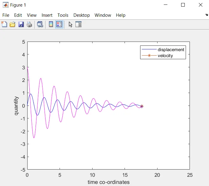
as , you can observe from the figure exponential decay of amplitude.

2. Simulation video of simple pendulum with underdamped condition:

Conclusion :

1. Plotted the velocity and displacement variations of simple pendulum with

underdamped condition.

2. Learned about damping.