Simulating the Rankine cycle using MATLAB

AIM: To simulate the Rankine cycle using MATLAB.

OBJECTIVES:

1. To calculate the state point of the Rankine cycle based on the user inputs.
2. To plot the corresponding T-s and H-s plot for the inputs given.

INTRODUCTION:

The Rankine cycle is an idealized thermodynamic cycle describing the process by which a certain heat engine, such as a steam turbine or reciprocating steam engine allows mechanical work to be extracted from a fluid as it moves between a heat source and heat sink.

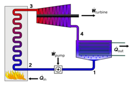
The processes involved in the working of the Rankine cycle are:

1-2 Isentropic Compression in the pump

Water enters the pump at state 1 as saturated liquid and is compressed isentropically to the boiler's operating pressure. The water temperature increases somewhat during this isentropic compression process due to the slight decrease in the specific volume of the water.

2-3 Constant pressure heat addition in a boiler

Water enters the boiler at stage 2 as a compressed liquid and leaves as superheated vapor at stage 3. The boiler is basically a large heat exchanger where the heat originated from combustion gases, nuclear reactors, or any other source is transferred to the water essentially at constant pressure.

3-4 Isentropic expansion in a turbine.

The superheated vapor at stage 3 enters the turbine where it expands isentropically and produces work by rotating the shaft connected to an electric generate. The pressure and the temperature of steam drop during this process to the value at stage 4 where the steam enters the condenser.

4-1 Constant pressure heat rejection.

Steam is condensed at constant pressure in the condenser, which is basically a large heat exchanger, by rejecting heat to a cooling medium. Steam leaves the condenser as a saturated liquid and enters the pump thus completing the cycle.

GOVERNING EQUATIONS

1. For boiler

`h_4 + Q_1 = h_1`

`Q_1 = h_1 - h_4`

2. For turbine

`h_1 = W_t + h_2`

`W_t = h_1 -h_2`

3. For condenser

`h_2 = Q_2 +h_3`

`Q_2 = h_2 - h_3`

4. For pump

`h_3 +W_p = h_4`

`W_p = h_4 - h_3`

5. Efficiency of rankine cycle

η = (Net work done)/(Heat supplied) = `= (W_P -W _T)/Q_s`

MATLAB CODE:

% Rankine cycle simulation 
close all
clear all
clc

% Different stage point 
% 1 = Turbine inle or boiler outlet ,  2 = Condenser inlet or turbine out 
% 3 = Pump inlet or condenser outlet , 4 = Boiler inlet or pump outlet 
% Input parameter 
%p1 = Turbine inlet pressure (bar)
%T1 = Temperature at the turbine inlet
%p2 = Turbine outlet pressure 
%Description about four process
fprintf('Process (1-2) - Isentropic expancion of the turbine \n');
fprintf('Process (2-3) - Isentropic heat rejection by the condenser \n');
fprintf('Process (3-4) - Isentropic compression in the pump \n');
fprintf('Process (4-1) - Isentropic Heat addition by the boiler \n');

% For input at stage I
p1 = input('Enter the pressure at the turbne Inlet (in bars):');
T1 = input('Enter the temperature at the turbne Inlet (in Degree):');
p2 = input('Enter the pressure at the turbne outlet (in bars):');

% calculating the state variables at all the stages 

%At point 1 
hg_1 = XSteam('hv_p',p1);
sg_1 = XSteam('sV_p',p1);
Tsat_P1 = XSteam('Tsat_p',p1);
Cp1_L = XSteam('CpL_p',p1);


%At point 2
hg_2 = XSteam('hv_p',p2);
sg_2 = XSteam('sV_p',p2);
Tsat_P2 = XSteam('Tsat_p',p2);
Cp2_L = XSteam('CpL_p',p2);

% At point 3 
hf_3 = XSteam('hL_p',p2);
sf_3 = XSteam('sL_p',p2);

% At point 4
hf_4 = XSteam('hL_p',p1);
sf_4 = XSteam('sL_p',p1);

% State variables at point 1 
fprintf('At stage 1 \n');
fprintf('p1 is :%f bar \n',p1);
fprintf('T1 is :%f degree C \n',T1);
h1 = XSteam('h_pT',p1,T1);
fprintf('h1 is :%f kJ/kg \n',h1);
s1 = XSteam('s_pT',p1,T1);
fprintf('s1 is :%f kJ/kg \n',s1);

% at stage variable point 2 
fprintf('At state 2 \n');
fprintf('p2 is : %f bar \n',p2);
% entropy remains same through out the turbine 
s2 = s1; 
fprintf('s2 is : %f kJ/kg \n',s2);
% calculation of dryness freaction 
if (s2 <= sg_2)
    x2 = (s2 - sf_3)/(sg_2 - sf_3);
else 
    x2 = 1;
end 
fprintf('x2 is : %f \n',x2);
if (x2<1)
    T2 = Tsat_P2;
else 
    %s2 = sg_2 + Cp2_V*(log(T2/Tsat_p2))   formula for calculating the temp
    %in superheated region
    T2 = (Tsat_P2 + 273.15)*exp((s2-sg_2)/Cp_2V);
    T2 = T2 - 273.15;
end
fprintf('T2 is :%f degree C \n',T2);
% for calculation of h2 
if (x2<1)
    h2 = hf_3+x2*(hg_2-hf_3);
else 
    h2 = XSteam('h_pT',p2,T2);
end
fprintf('h2 is :%f kJ/kg',h2)

% state variable at point 3

fprintf('At state 3 \n');
p3 = p2;
fprintf('p3 is :%f bar \n',p3);
V3 = XSteam('vL_p',p3);
T3 = Tsat_P2;
fprintf('T3 is : %f degree C \n',T3)
h3 = hf_3 ;
fprintf('h3 is : %f kJ/kg |n',h3);
s3 = sf_3;
fprintf('s3 is : %f kJ/kgk \n ',s3);

% state variable at point 4 
fprintf ('At state 4 \n')
p4 =p1;
fprintf('p4 is :%f bar \n ',p4);
% tsentropic pumping process 
s4 = s3;
fprintf('s4 is : %f kJ/kgk \n',s4);
T4 = XSteam('T_ps',p4,s4);
fprintf('T4 is :%f degree \n',T4);

W_P = V3 * (p4-p3)*100;
h4 = W_P +h3;
fprintf('h4 is :%f kJ/kg \n',h4);

% calculation of the other parameters 

%work done by turbine 
W_T = h1 - h2;
fprintf('Work done by turbine is : %f kJ/kg \n',W_T);
fprintf('Work done by pump is : %f kJ/kg \n',W_P);

% Net woek done
Wnet = W_T - W_P;
fprintf('Net Work done is : %f kJ/kg \n',Wnet);

% net heat supplied
Qin = h1 - h4;

% Thermal efficiency 
eff_thermal = Wnet/Qin;
fprintf('thermal efficiency is : %f \n',eff_thermal);

% back work ratio
b_w_r = (W_P/W_T);
fprintf('back work ratio is: %f \n',b_w_r);
%work ratio 
w_r = (Wnet/W_T);
fprintf('Work ratio is: %f  \n',w_r);
% Summation 
fprintf('Back work + work ratio is: %f \n',(b_w_r+w_r));

% heat rate and specific steam comsumption 
h_r = (1/eff_thermal);
fprintf('heat rate is : %f  kJ/kWs  \n ',h_r);
ssc = (1/Wnet);
fprintf('Specific steam cosumption : %f  kJ/kWs  \n ',ssc);

temperature = linspace (0,T1,5000);
for i = 1:length (temperature)
    H_l(i) = XSteam('hL_T',temperature(i));
        H_v(i) = XSteam('hV_T',temperature(i));
            S_l(i) = XSteam('sL_T',temperature(i));
                S_v(i) = XSteam('sV_T',temperature(i));
end

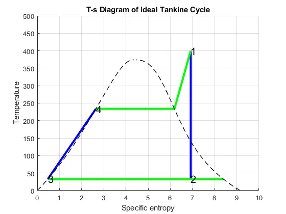
%plotting T-s diagram
figure (1)
hold on 
plot([s1 s2], [T1 T2], 'color','b','linewidth',3)
plot([s2 sg_2], [T2 Tsat_P2], 'color','g','linewidth',3)
plot([sg_2 s3], [Tsat_P2 T3], 'color','g','linewidth',3)
plot([s3 s4], [T3 T4], 'color','b','linewidth',3)
plot([s4 sf_4], [T4 Tsat_P1], 'color','b','linewidth',3)
plot([sf_4 sg_1], [Tsat_P1 Tsat_P1], 'color','g','linewidth',3)
plot([sg_1 s1], [Tsat_P1 T1], 'color','g','linewidth',3)

text(s1,T1,'1','Fontsize',15)
text(s2,T2,'2','Fontsize',15)
text(s3,T3,'3','Fontsize',15)
text(sf_4,Tsat_P1,'4','Fontsize',15)

plot(S_l,temperature,'black','linestyle','--','linewidth',1)
plot(S_v,temperature,'black','linestyle','--','linewidth',1)

axis([0 10 0 500])
title('T-s Diagram of ideal Tankine Cycle')
ylabel('Temperature')
xlabel('Specific entropy')
grid on

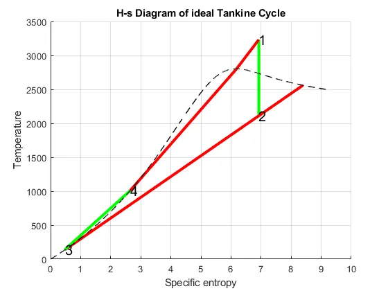
%plotting T-s diagram
figure (2)
hold on 
plot([s1 s2], [h1 h2], 'color','g','linewidth',3)
plot([s2 sg_2], [h2 hg_2], 'color','r','linewidth',3)
plot([sg_2 s3], [hg_2 h3], 'color','r','linewidth',3)
plot([s3 s4], [h3 h4], 'color','g','linewidth',3)
plot([s4 sf_4], [h4 hf_4], 'color','g','linewidth',3)
plot([sf_4 sg_1], [hf_4 hg_1], 'color','r','linewidth',3)
plot([sg_1 s1], [hg_1 h1], 'color','r','linewidth',3)

text(s1,h1,'1','Fontsize',15)
text(s2,h2,'2','Fontsize',15)
text(s3,h3,'3','Fontsize',15)
text(sf_4,hf_4,'4','Fontsize',15)

plot(S_l,H_l,'black','linestyle','--','linewidth',1)
plot(S_v,H_v,'black','linestyle','--','linewidth',1)


title('H-s Diagram of ideal Tankine Cycle')
ylabel('Temperature')
xlabel('Specific entropy')
grid on

EXPLANATION OF CODE:

1. To initiate the program we will first have the input parameters to the program that are p1, T1, p2.
2. Next from the Xsteam library to get the steam table data of water, all the properties like enthalpy, entropy, specific heat, saturation temperature, etc.
3. These variables are used further to calculate work done by pump, work done by the turbine, net work done, back work ratio efficiency of the cycle.
4. To plot the water diagram for the above data an array is created from 0 to temperature value T1 and using the for loop to state all the variables.
5. Next, all the values are plotted using the plot command and are marked using the text command.

OUTPUT:

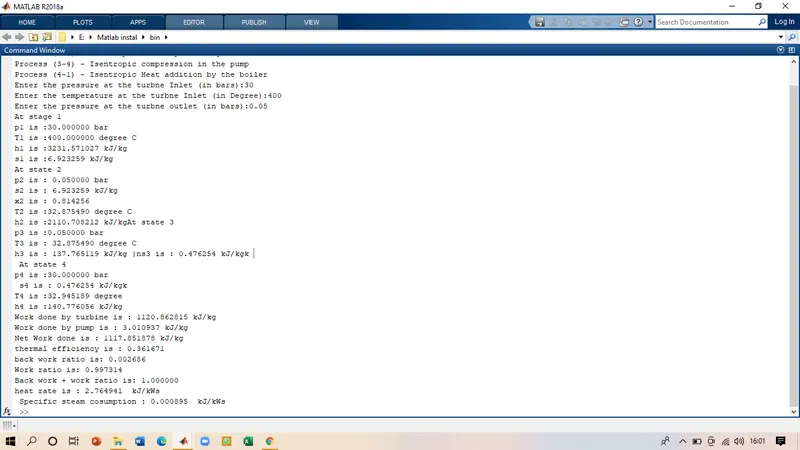
Command window output

The input for the program were given as p1 = 30 bars , T1 = 400 degree C, p2 = 0.05 bars

The T-s plot for the cycle is

H-s plot for the cycle

CONCLUSION

Here we can see that we have successfully calculated all the properties for the Rankine cycle and have plotted the T-s and H-s diagram for the same. Using this program we can calculate the properties of water operated rankline cycle for any given input conditions.