SIMULATING THE FLOW OF AIR THROUGH A CHANNEL USING CONVERGE CFD
Aim :
To simulate the flow of air through a channel using converge CFD by using 3 different grid sizes and comparing the results by generating plots and animations for velocity and pressure contours.
Three different base mesh sizes are
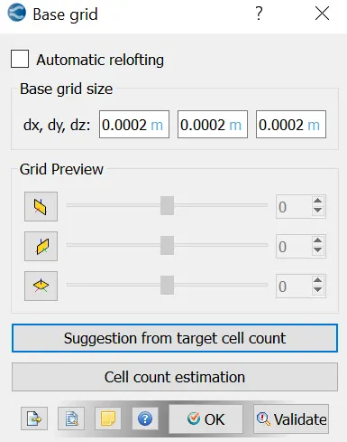
- dx= 2e-4 m dy = 2e-4 m dz= 2e-4 m
- dx= 1.5e-4 m dy = 1.5e-4 m dz= 1.5e-4 m
- dx= 2e-4 m dy = 2e-4 m dz= 2e-4 m
Introduction :
conduit is a natural or artificial channel through which something (such as a fluid) is conveyed. Flow through conduits are basically two types.
- Open channel flow : In this type of flow is only for liquids. Here flow has only one free surface i.e surface exposed to atmosphere
- Closed conduit flow : Example pipe flow, Flow of air through air duct, closed rectangular channel
A closed channel flow with channel cross section H x W (Height x Width) where the height is fixed and the width is infinite in other words, air flow between two parallel plates of infinite width i.e simulation is done only on a 2D flow basis in which pressure and velocity profiles are monitored along the height of the channel at different points along the length of the channel.
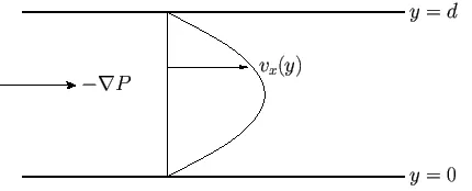
Fluid flow through conduits like channels, pipes and air ducts are always in contact with the rigid boundaries. At the point of contact the flow velocity is zero or the fluid is at rest. At the centre the flow velocity is maximum. As we move from the centre to the rigid boundaries, the velocity decreases from maximum to zero. Because of the fluid viscosity, fluid layers at the boundary resist the motion of fluid layers at the centre and therefore velocity changes from the centre to the boundary and it has a parabolic profile.
Theory
The results of a CFD simulation are obtained by solving the Navier-Stokes equations. These are 5 equations, continuity, momentum (3 equations), and energy equations. The continuity and momentum equations are solved for all types of flow problems and the energy equation can be used only when heat transfer is taking place to speed up the simulation. These equations are numerically solved in computers using algorithms like SIMPLE and PISO.
We assume that there is no heat transfer happening and the flow is incompressible. So we have 4 equations (Continuity and 3 momentum equation) to solve and 4 unknowns (Pressure and Velocity in 3 directions).
Continuity Equation:
`{delu}/{delx} + {delv}/{dely} +{delw}/{delz} =0`
X momentum :
`rho{Du}/{Dt} = -{delp}/{delx} + munabla^2u + pf_x`
Y Momentum :
`rho{Dv}/{Dt} = -{delp}/{dely} + munabla^2v + pf_y`
Z Momentum :
`rho{Dw}/{Dt} = -{delp}/{delz} + munabla^2w + pf_z`
Where u, v and w are the velocities in x, y and z directions respectively
`rho` is the density and p is the pressure, `nabla = del/{delx} + del/{dely} +del/{delz}`
These equations are solved using the pressure correction method by using the SIMPLE and PISO algorithms.
Here we can see that all 4 equations have a velocity term and only 3 equations have a pressure term so we need to use the pressure correction method.
SIMPLE
SIMPLE stands for Semi-Implicit Method for Pressure Linked Equations. Here the first step is the predictor step where the pressure is guessed and in the next step the corrections are applied and is called as the corrector step. In each iteration there is one predictor step and one corrector step. SIMPLE algorithm is used for steady state problems.
The pressure at step n+1 is
`p^{n+1} = p^{******} + r*p^n`
where r is an under-relaxation factor whose value can vary from 0 to 1 to obtain a stable solution and n indicates the current iteration at which the solution has progressed.
PISO
PISO stands for Pressure Implicit with Splitting of Operator. It is generally used for transient solutions but can be used for steady solutions as well. PISO is similar to SIMPLE except that SIMPLE uses one corrector step and PISO uses 2 or more corrector steps. And PISO allows larger timesteps without affecting the stability of the solution
Case setup :
1. Creating the geometry :
Go to geometry editing tool box > select create > select shape tab > select box
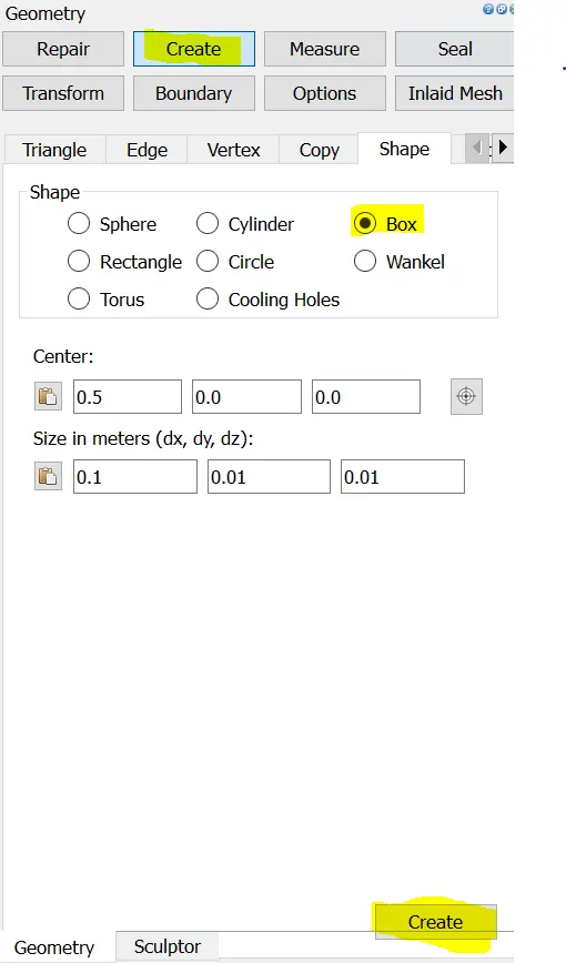
dx,dy and dz are the lengths in x,y and z directions respectively
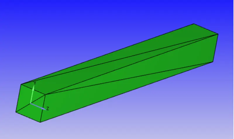
2. Creating boundaries for the geometry :
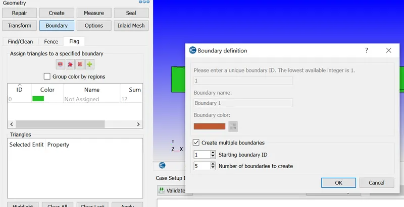
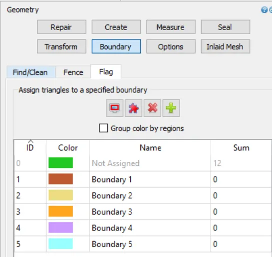
5 boundaries will be created with default names
3. Assigning boundaries to faces of the geometry
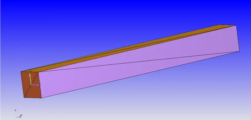
To assign a boundary to a face select the 2 triangles (of the face) then select the boundary name and press apply
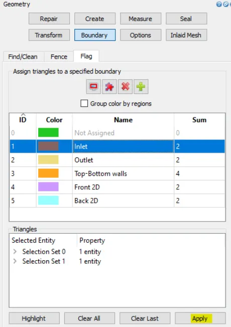
4. Checking the orientation of normals :
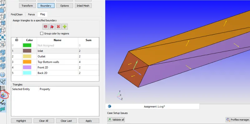
Enable the normal by clicking the Normal Toggle icon in the left panel. All the normals are pointing away from the fluid so this has to be transformed. select any one triangle whose normal is pointing away from the fluid and in geometry editing tool box select transform , under normal select propagate change from a single triangle and apply.
5. Running a Diagnosis check for any Geometry errors
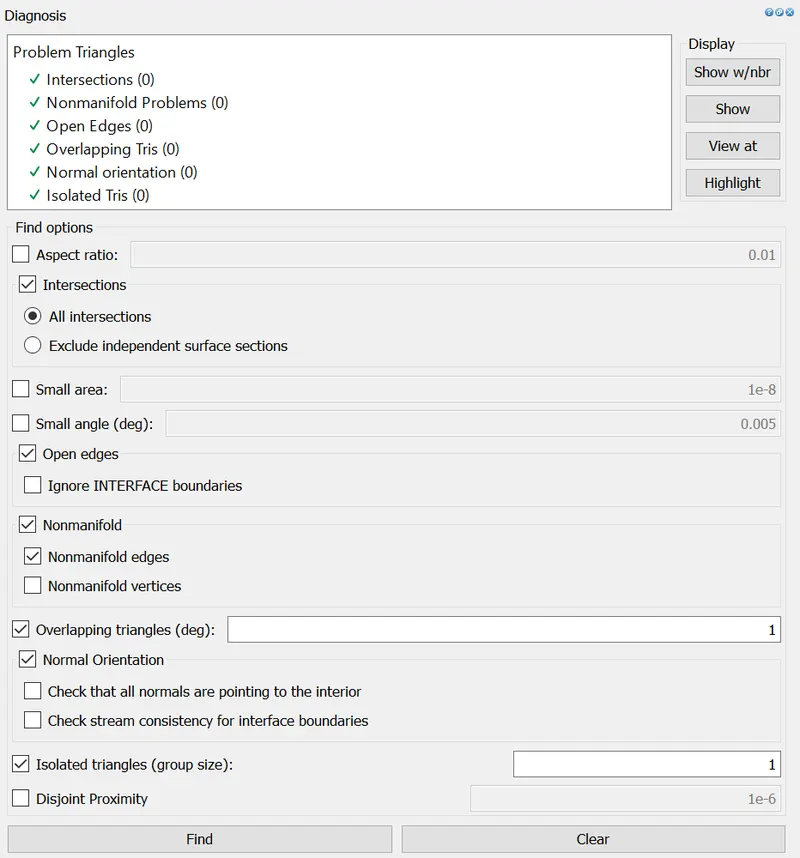
As all parameters are green checks there are no errors in geometry
6. Case setup :
6.1 Application type :
on right panel go to the case set up tab
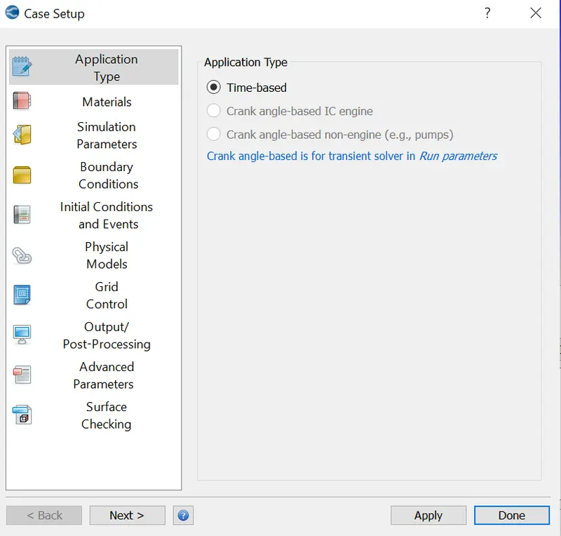
As it is a time based application click and apply
6.2 physical models
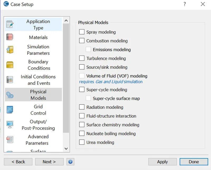
select physical models and disable turbulence modelling and click apply
6.3 Materials :
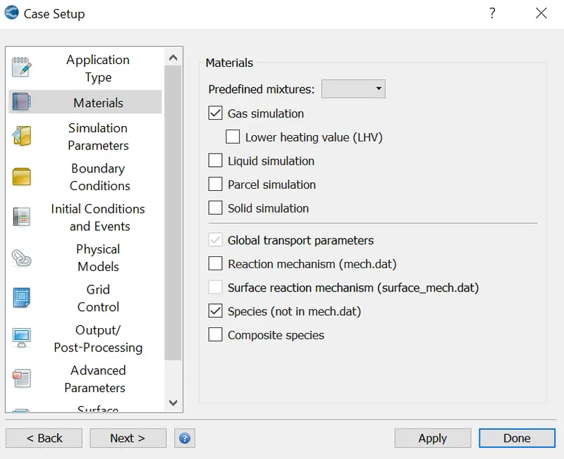
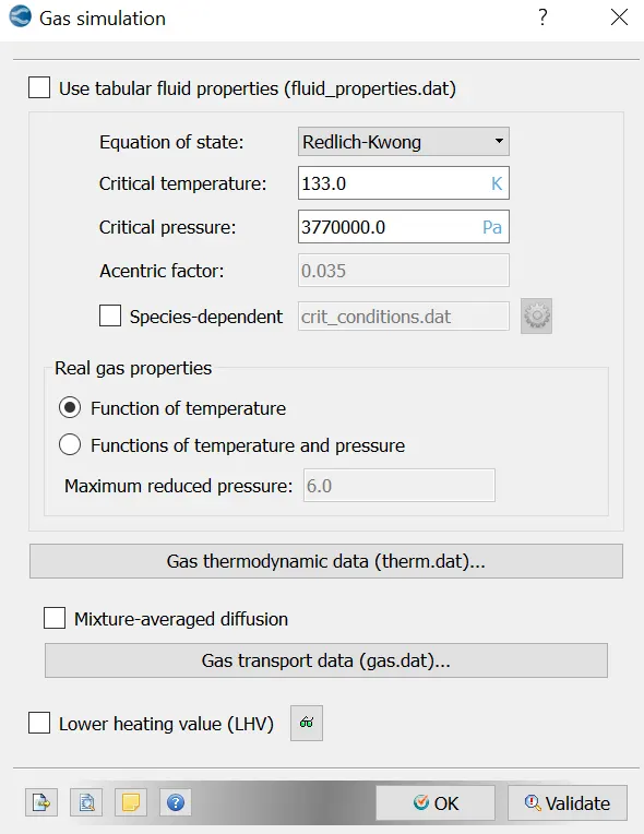
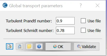
select materials and uncheck the reaction mechanism as we are not simulating any reactions then select predefined mixtures as Air and then press apply.
Species :
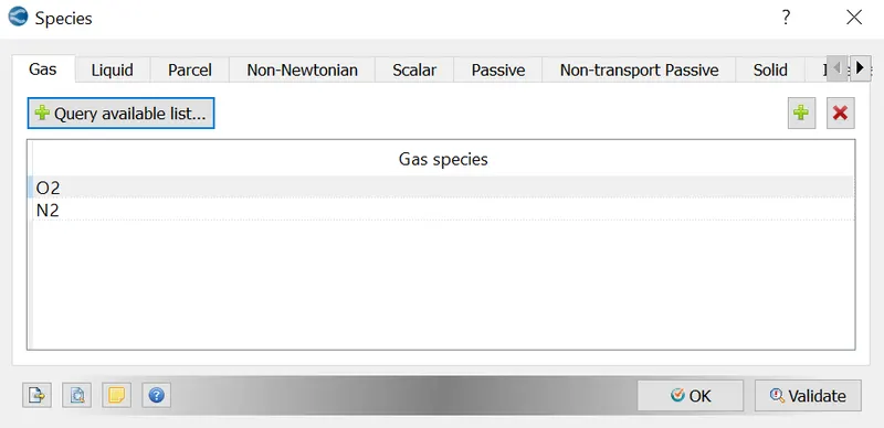
In species add O2 and N2 and press ok.
6.4 Run Parameters
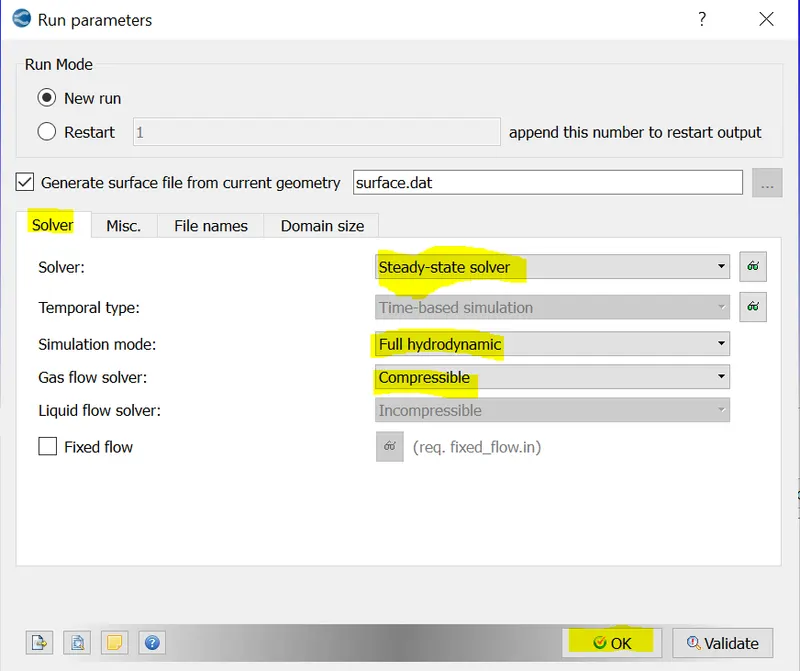
under solver tab press steady state solver and select full hydrodynamic simulation mode.
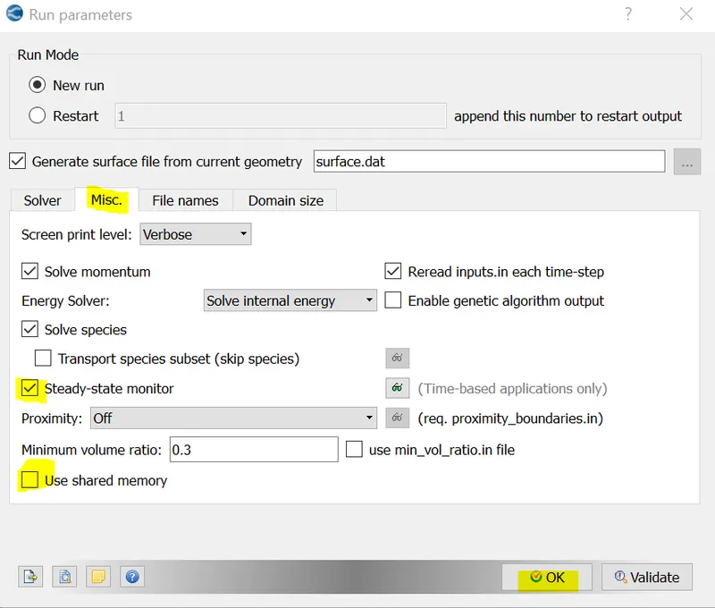
under misc tab uncheck use shared memory box and check steady state monitor
6.5 Simulation time parameters :
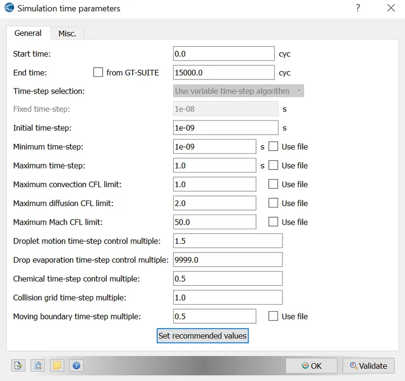
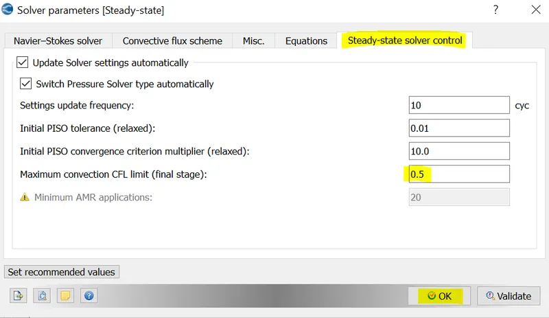
6.6 Solver parameters :
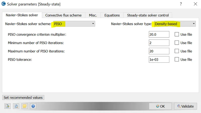
select the Navier stokes solver type as density based
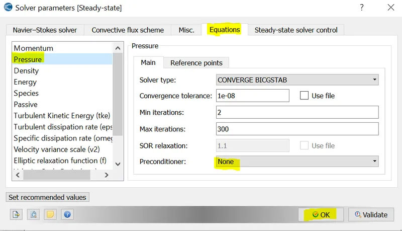
Under Equations tab set preconditioner for pressure as none
6.7 Regions and Initializations :
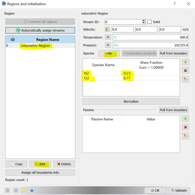
This defines a volumetric region with initial conditions like initial pressure, initial temperature, velocity and species concenration( O2 77% and N2 23% )
6.8 Boundary conditions :
Inlet :
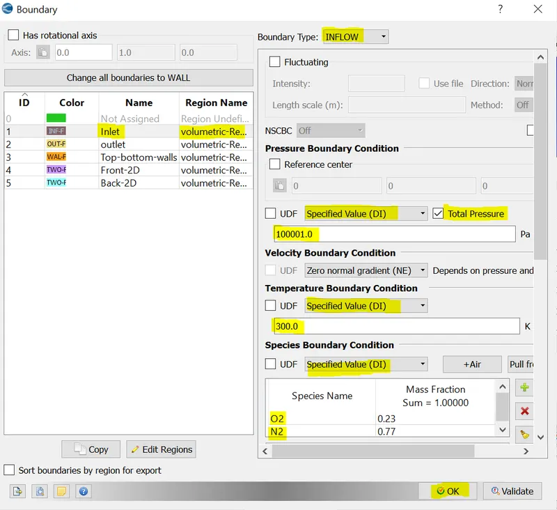
For inlet select the pressure boundary condition as a specified value of 100001 pa and select air for species boundary condition
Outlet :
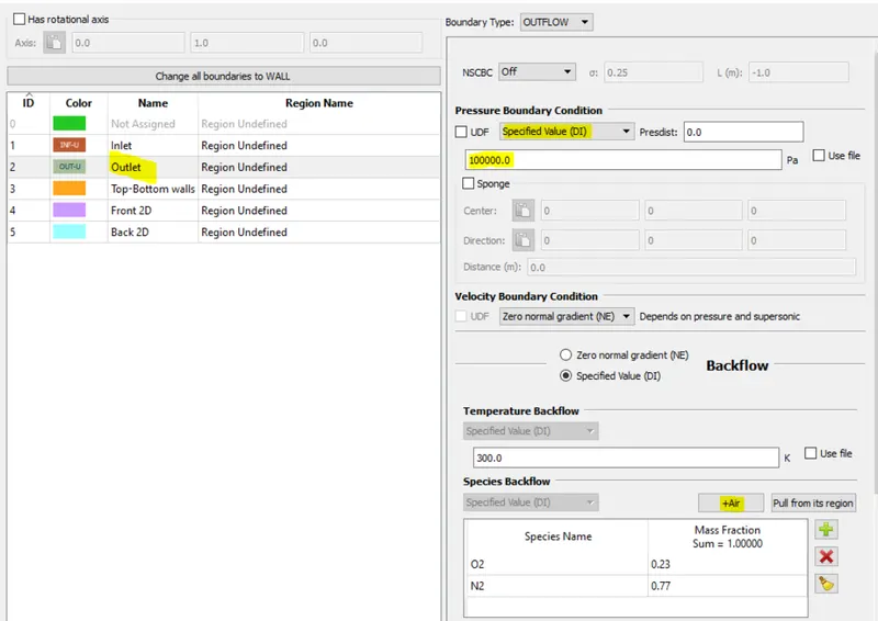
select the outlet pressure as 100000 pa and for species back flow select air
Top and bottom walls :
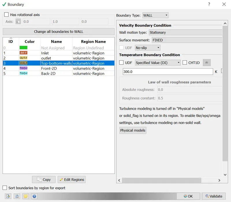
select the top and bottom boundary as wall type with no slip boundary condition. No slip means flow velocity at the boundary is zero. Keep the temperature as specified value as 300 K
Front 2D and back 2D :
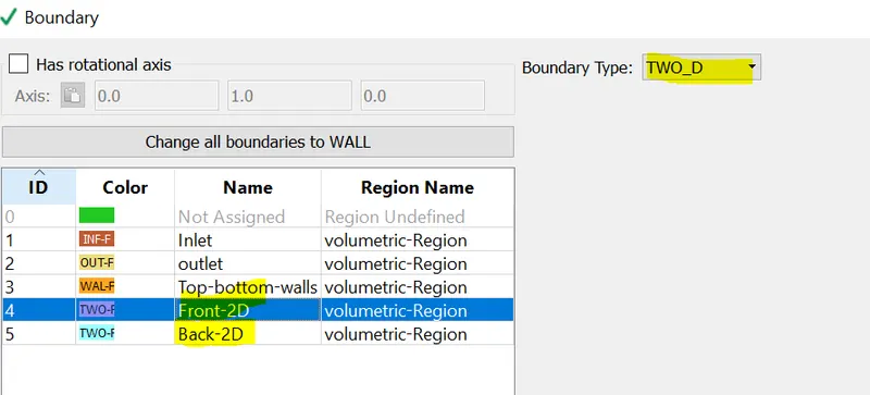
Select the boundary type for front and back faces as 2D as we are simulating 2D flow.
6.9 steady state monitor :
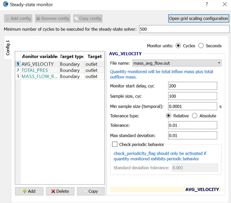
select staedy state monitor and a new pop out window will appear. select add configuration button then click on add button
select the required monitor variables, Target type as boundary and Target as outlet because an inlet velocity boundary condition was given.
Then on the right side set the monitor units as cycles. The units are selected as cycles if the simulation is steady state and seconds if the simulation ios transient.
Monitor delay ensures that simulation runs for a minimum number of cycles or seconds before the variable can be monitored. set this parameter as 200.
Sample size indicates the number of cycles or seconds after which the variable is checked for convergence. set this parameter as 100.
The solution is said to be converged if the average change in the variable value over a number of cycles is less than the tolerance value.
6.10 Base Grid:
6.11 Post variable selection :
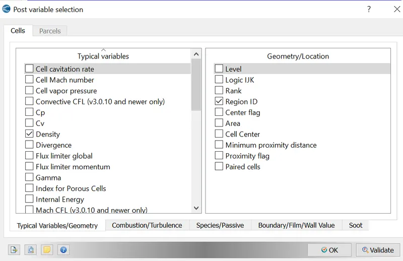
check the required varibles
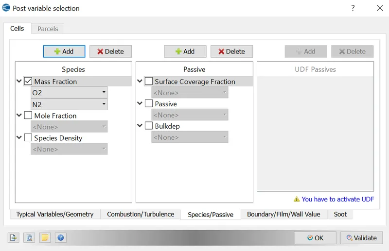
In the species tab add O2 and N2 mass fractions
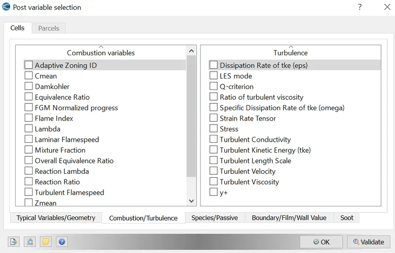
Deselct all the check boxes under the combustion/Turbulence tab inside the turbulence window.
6.12 Output files :
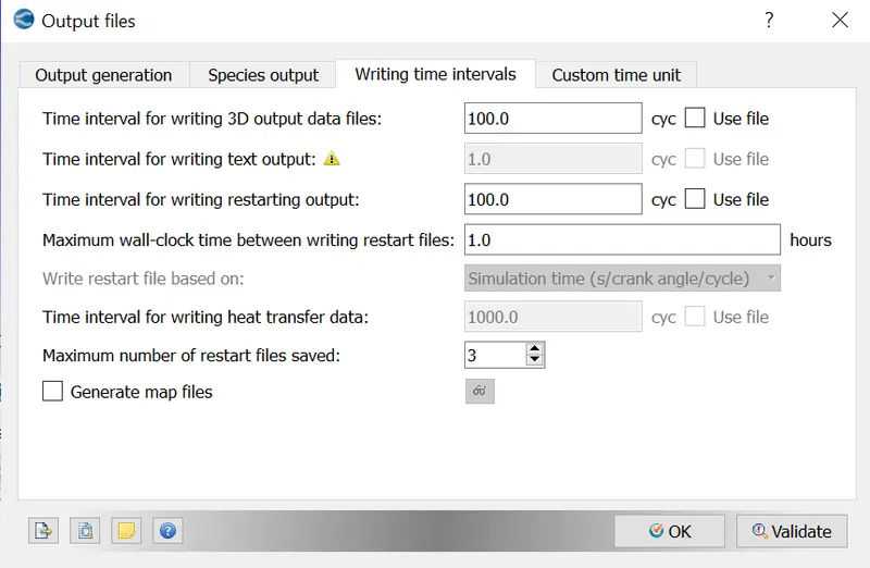
There are 15000 cycles for this simulation and we have set the time interval for writing 3D output data files as 100 cycles. It means after every 100 cycles converge will write the output data file so in total there will be 15000/100 =150 output files. the option for time interval for writing the text output is not selected because the steady state monitor iis enabled. So converge will write the text output for every cycle.
Time interval for writing retstrating o/p is the number of cycles after which converge will write a simulation restore point so that when there is a power failure the restart file can be used to resume the simulation from the point at which there is a power failure.
7. Exporting all the input files in to folder :
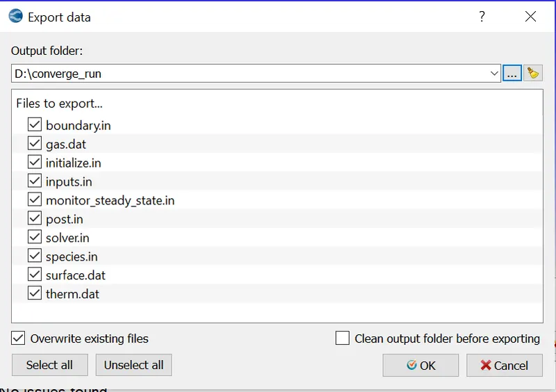
Go to file menu and select export option and export all the input files to the desired folder.
8. Running the simulation in Cygwin

Navigate to the folder in the cygwin where the input files are dumped and execute the above command. Its a parallel computation as it is running on the 4 processors the path where the convege intel mpi executable is located is pasted and the log file is created to check the output log messages.
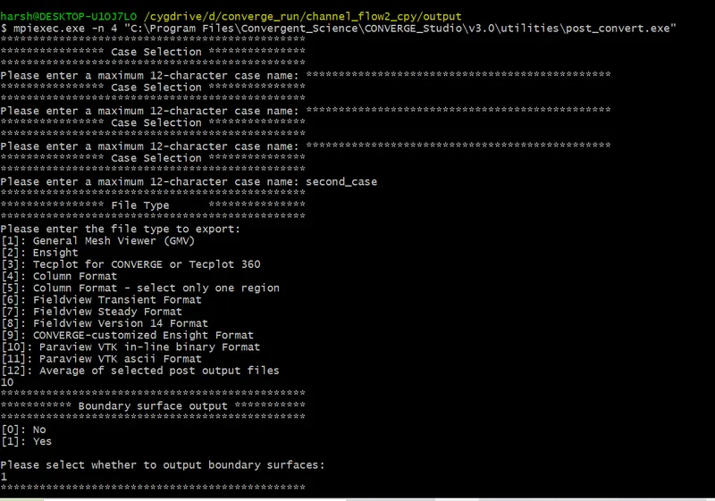
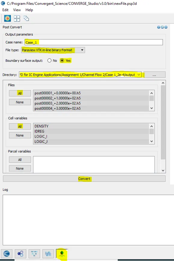
9. Post converting all the output files
post converting can be done by using cygwin and also by using converge but parallel post processing can be done only by cygwin
Using cygwin:
Using converge :
10. Launching paraview
Results for simulation of case 1 (dx=dy=dz=2e-4)
Mesh

Velocity and Pressure Contours for Case 1 (dx = dy = dz = 2e-4)
Velocity Contour Plot
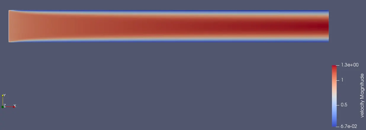
Comments: As we can see from the contour plot that the velocity profile is flat in the entrance region and as the flow develops the velocity increases in the central region and decreases in the peripheral region. On the right end of the image (the outlet) flow is fully developed and velocity is maximum in the central region (near outlet).
Pressure Contour Plot
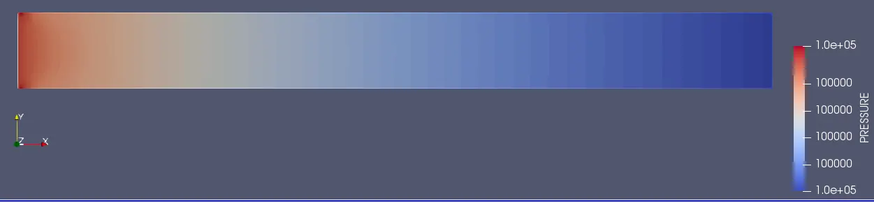
Comments: Pressure decreases from 100001 Pa at the inlet to 100000 Pa to the outlet. Air flows because of the pressure difference.
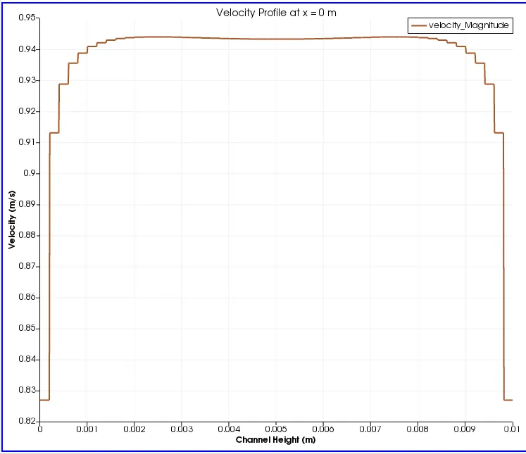
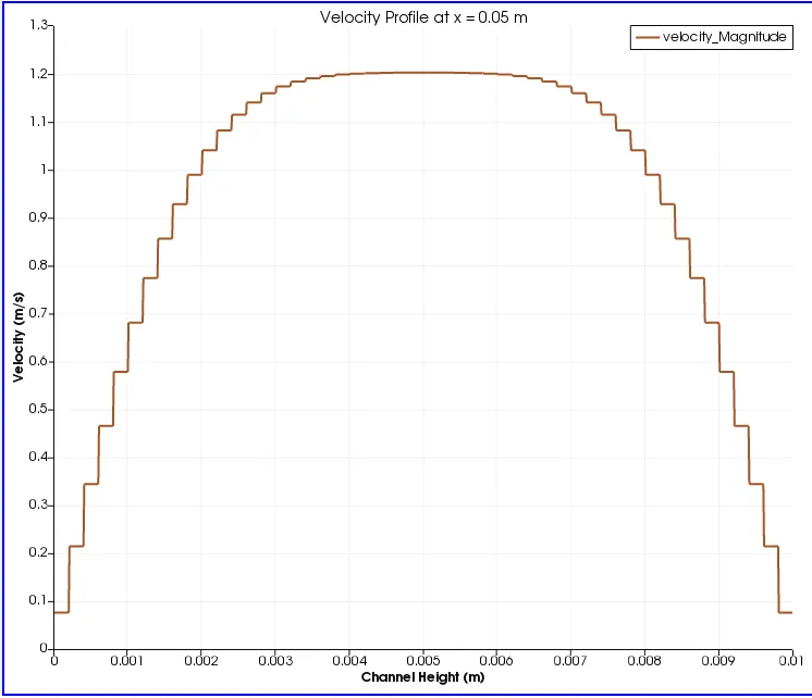
Velocity Profile Plots
at x = 0
at x = 0.05
at x = 0.1
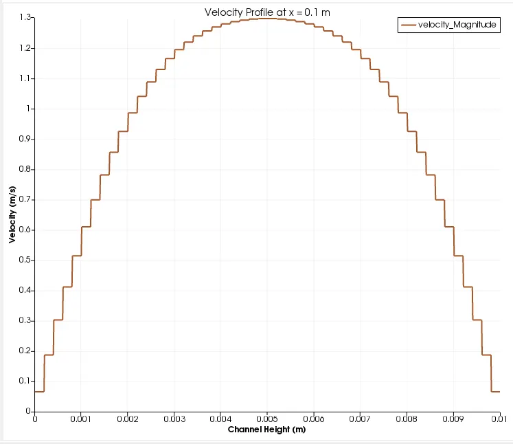
Comments:
At inlet the velocity profile is flat and max velocity is 0.943 m/s,
Mid-way of the channel length the max velocity is 1.2 m/s and velocity profile is partially developed
At the outlet of the channel the max velocity is close to 1.3 m/s and velocity profile is fully developed and parabolic.
Pressure Profile Plot along the length of the channel
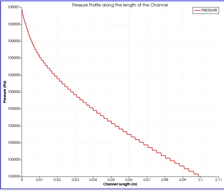
Comments:
A steep slope curve at the entrance region followed by a linear pressure drop at the fully developed zone. This is the expected output as the pressure gradient is always higher in the entrance region than the fully developed region similar to that in case of a pipe flow.
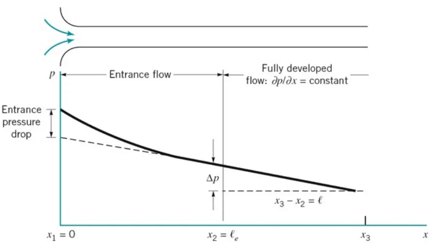
As the flow develops, the flow velocity is accelerated in the central region and retarted near the top and bottom walls, because of this relative motion between fluid layers and difference in acceleration the pressure drop per unit length is higher in the entrance region than in fully developed region.
Pressure Plot in converge
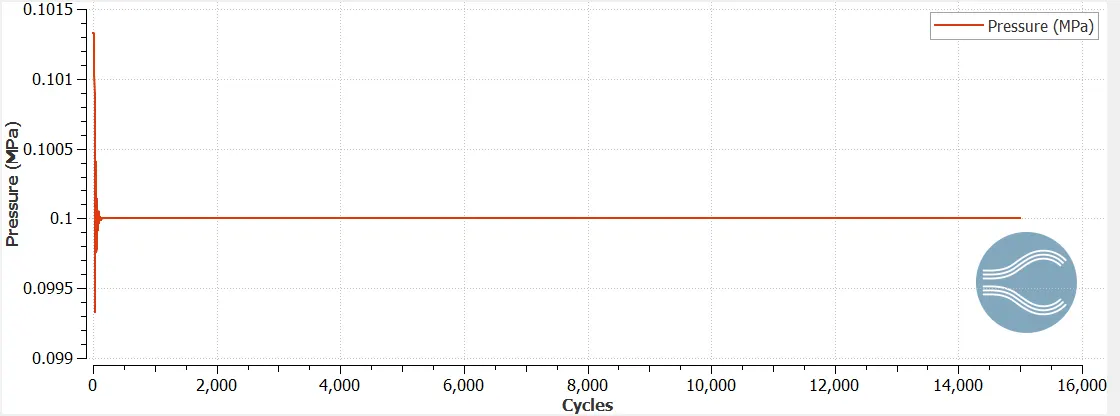
Total Number of Cells Count in ParaView
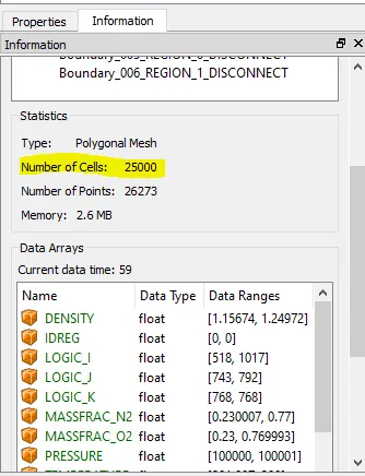
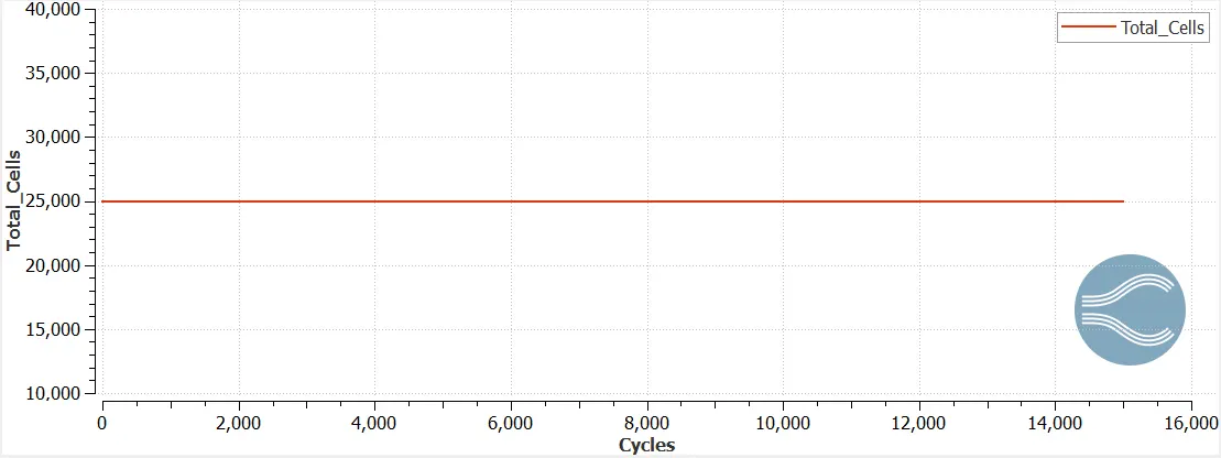
Total number of cells = 25000
Plot of Mass Flow Rate vs Number of Cycles
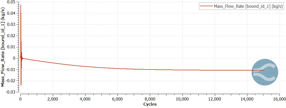
At Inlet
At Outlet
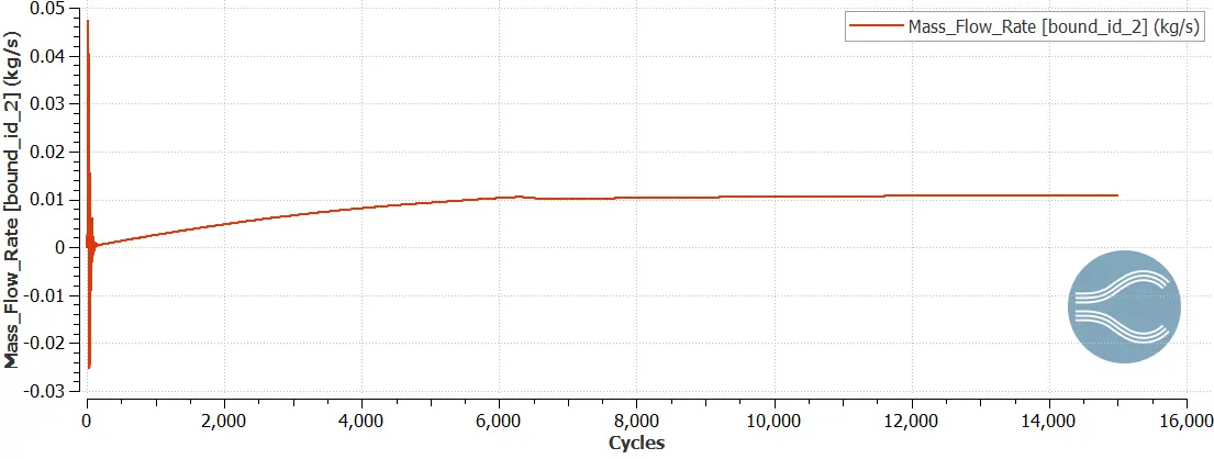
Comments: Mass flow rate at inlet = Mass flow rate at outlet = 0.0108 kg/s
As we can see from the plots that the mass flow rate values have converged to 0.0108 kg/s. And the mass flow rate is negative for inlet because the mass flows in a direction opposite to the inlet boundary plane.
Results of Simulation for Case 2 (dx = dy = dz = 1.5e-4)
Mesh

Velocity and Pressure Contours
Velocity Contour Plot
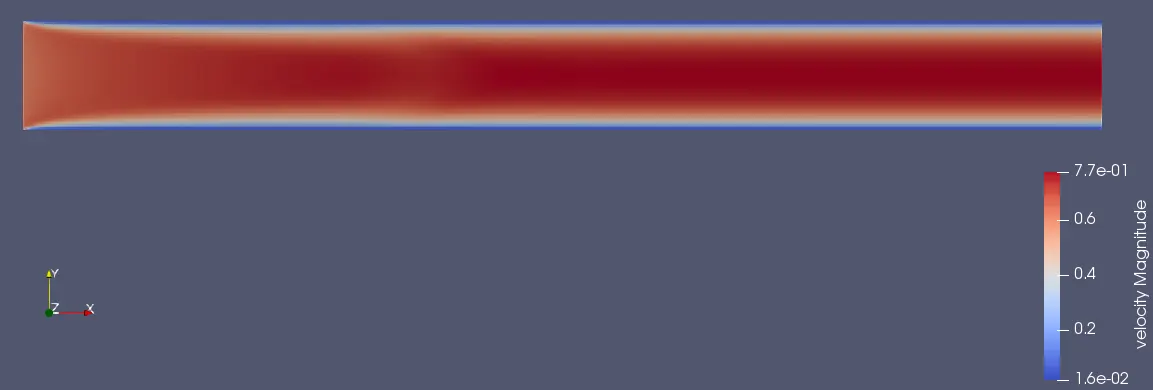
Comments: As we can see from the contour plot that the velocity profile is flat in the entrance region and as the flow develops the velocity increases in the central region and decreases in the peripheral region. On the right end of the image (the outlet) flow is fully developed and velocity is maximum in the central region (near outlet).
Pressure Contour Plot
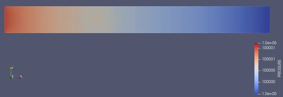
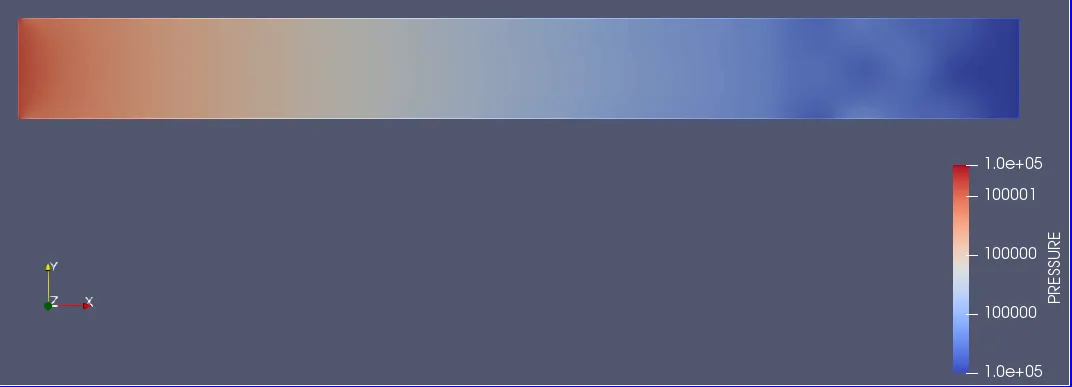
Pressure linearly decreases from 100001 pascals to 100000 pascals.
Velocity Profile Plots
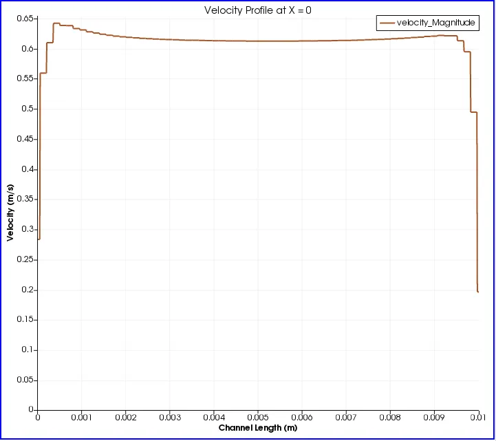
at x = 0
at x = 0.05
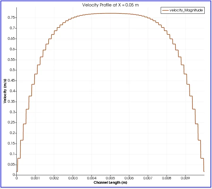
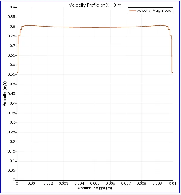
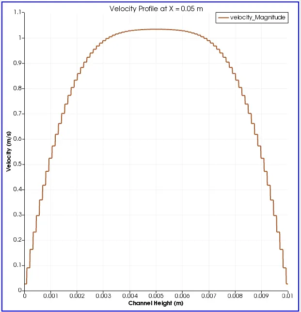
Comments: As we move towards the +X axis the velocity in the central region (midway between the top and bottom planes) the veocity acceletates and in the region close to the top and bottom plates the velocity gets retarded.
Pressure Plot in Converge
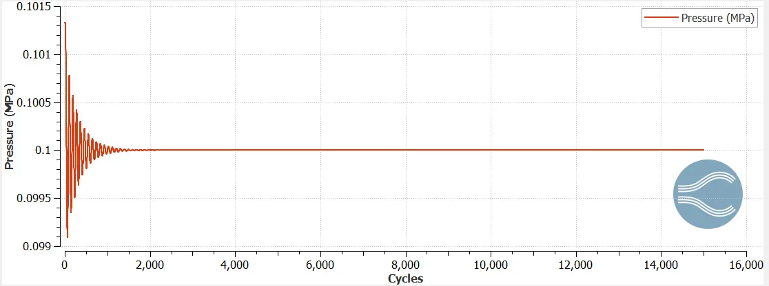
Comments: From the above plot we can see how pressure converges after a certain number of cycles.
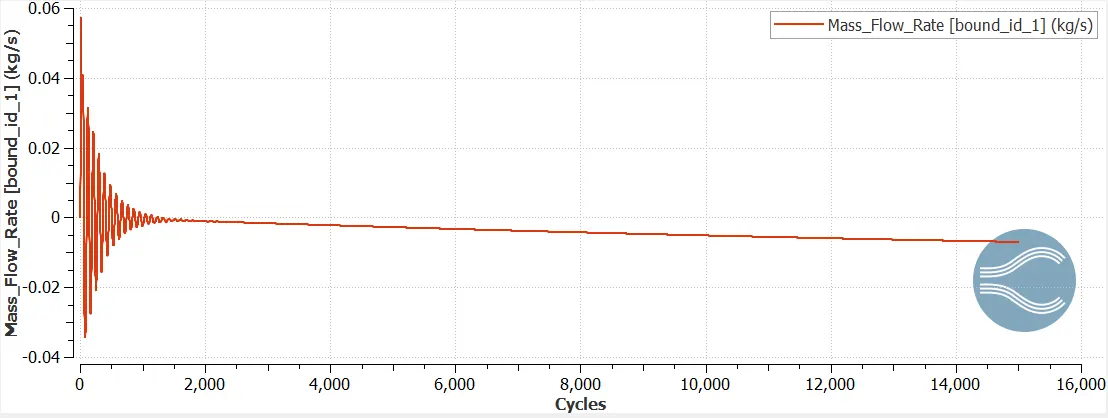
Plot of Mass Flow Rate vs Number of Cycles
At Inlet
At Outlet
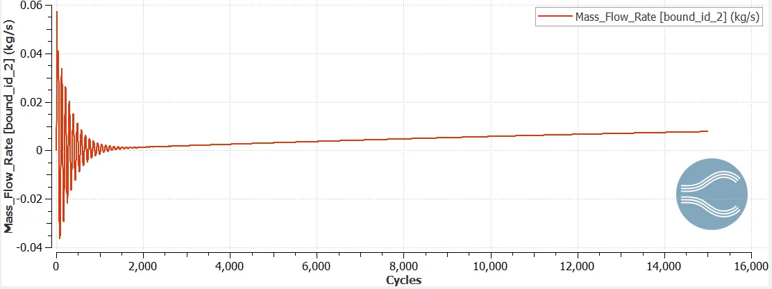
Comments: Mass flow rate converges after a certain number of cycles.
Total Number of Cells Count in ParaView
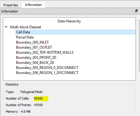
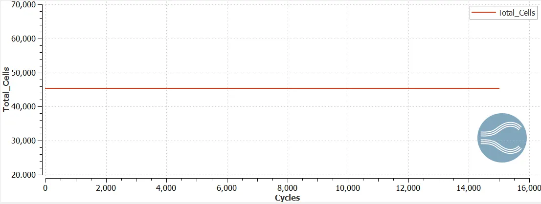
Total number of cells = 45420
Results of Simulation for Case 3 (dx = dy = dz = 1.2e-4)
Mesh

Velocity and Pressure Contours
Velocity Contour Plot
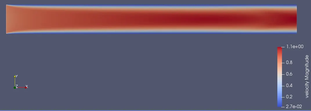
Comments: As we can see from the contour plot that the velocity profile is flat in the entrance region and as the flow develops the velocity increases in the central region and decreases in the peripheral region. On the right end of the image (the outlet) flow is fully developed and velocity is maximum in the central region (near outlet).
Pressure Contour Plot
Velocity Profile Plots
at x = 0
at x = 0.05
Pressure Plot in Converge
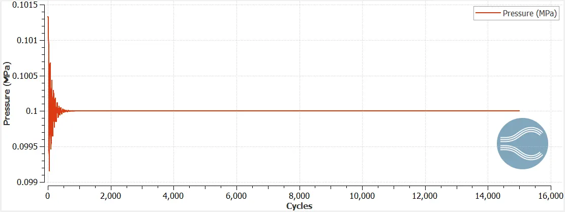
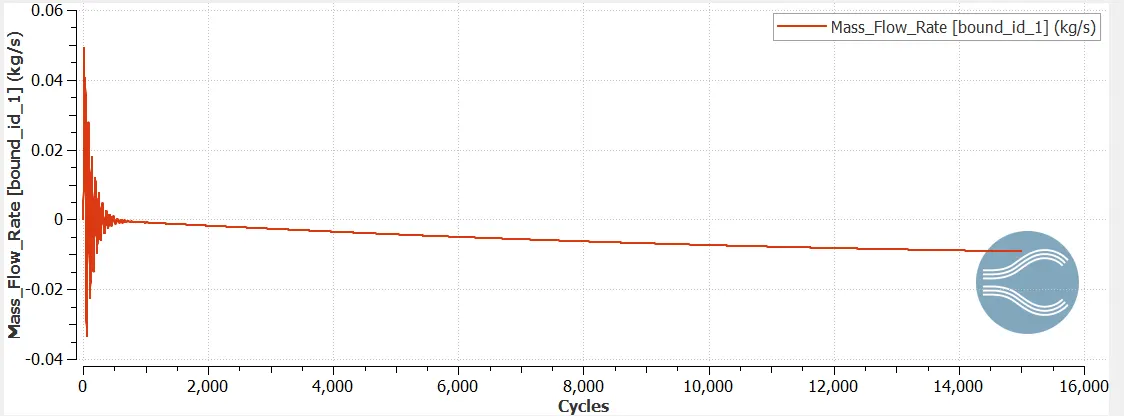
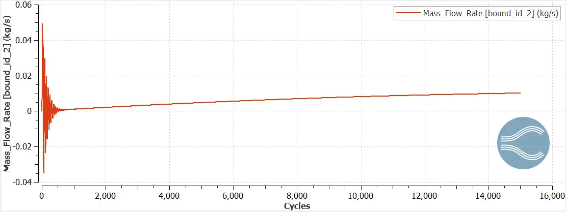
Plot of Mass Flow Rate vs Number of Cycles
At Inlet
At Outlet
Total Number of Cells Count in ParaView
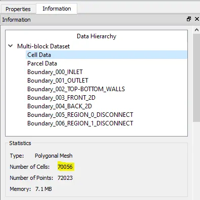
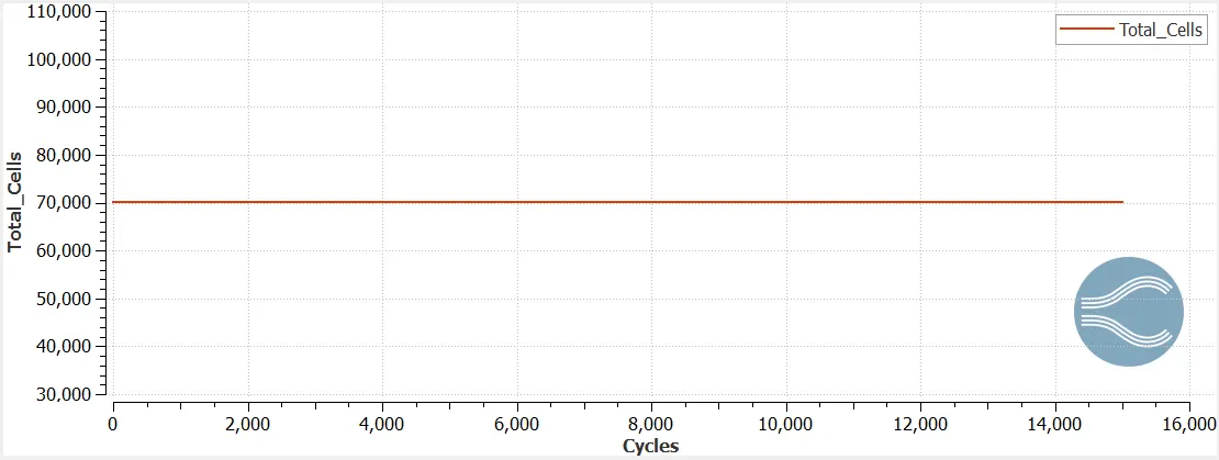
Total number of cells = 70056
Animation of how the velocity contour plot converges
At time = 0:00 shows the initial velocity contour plot, velocity is zero everywhere in the entire domain. As time progresses the velocity starts to increase. After 12 seconds in the video, the velocity contour has completely converged and that contour plot shows how the velocity changes from the entrance of the channel to the outlet. At the entrance the velocity profile is flat and as we move towards the outlet the velocity increases in the central region and decreases in the region near the top and bottom channel faces.
Conclusion:
1. As we decrease the mesh size, the results become more accurate and it produces smooth plots but the computation time increases drastically.
2. As we decrease the mesh size, Converge decreases the time step as well to maintain the CFL number and to keep the solution stable. Because of that the number of cycles required for convergence increases which again increases the computation time.